Displaying a Dependent Drop-Down List

In this example we are going to create two drop-down lists.
Depending on the value selected in the first drop-down list will determine what values are displayed in the second.

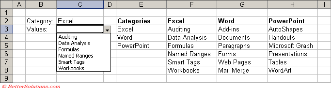Create a table with all the corresponding values
In this example we are going to have 3 categories (Excel, Word and PowerPoint) each one has 6 different values.

Create the Named Ranges

Highlight the cells "E3:E5".
Select (Insert > Name > Define) and type the name "Category".

Highlight the cells "F3:F8". Select (Insert > Name > Define) and type the name "Excel".
Highlight the cells "G3:G8". Select (Insert > Name > Define) and type the name "Word".
Highlight the cells "H3:H8". Select (Insert > Name > Define) and type the name "PowerPoint".

Enter the Criteria for the first Drop-Down List

Select the cell you want the first drop-down list to appear in, in this case cell "C2".
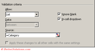
Select (Data > Validation) and select the Settings tab.
In the "Allow" drop-down box select "List".
In the "Source" box enter the formula "=Category" to refer to the named range that you created earlier.

Enter the Criteria for the second Drop-Down List

Select the cell you want the first drop-down list to appear in, in this case cell "C3".
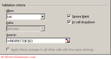
Select (Data > Validation) and select the Settings tab.
In the "Allow" drop-down box select "List".
In the "Source" box enter the formula "=INDIRECT($C$2)" to refer to the named range that you created earlier.
The INDIRECT function can also be used to

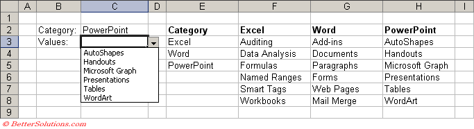
Displaying the PowerPoint Values

You now have two dependent drop-down list boxes where the values in the second list depend on the selection made in the first drop-down.

Drop-Down List with Spaces

Remember that named ranges cannot contain spaces so if you have items that are more than one word in the first drop-down list, you will need to remov the spaces when creating the corresponding supporting named ranges.
You can easily remove the spaces from the selected item by using the SUSTITUTE function.
In this situation modify the source formula to be the following:
=INDIRECT(SUBSTITUTE(C2," ",""))
SS

If your first drop-down list contains some characters which are not allowed in ranges named then this can be overcome by using a simple lookup table.
Create a named range for this table called DropDownLookup
SS
In this situation modify the source formula to be the following:
=INDIRECT(VLOOKUP(C2,DropDownLookup,2,0))
SS

Dynamic Drop-Down List

The INDIRECT function is very usefult for ??
If you want to create dynamic second drop-down lists then you will need to use the familiar OFFSET and COUNTA functions in your source formula.
You can either define the supporting named ranges to be dynamic or you can just use a dynamic formula in your source formula.
SS