Formatting

Applying formatting to your worksheets will make them easier to read and interpret your data.
You can apply formatting to cells very quickly by selecting the cells or range of cells and choosing the appropriate commands
The (Format > Cells) dialog box gives you access to most of the formatting options including changing fonts, character formatting, cell alignment and applying borders and shading.
Borders are an easy way to separate and define different areas on a worksheet.
There are an enormous number of formatting options on the Formatting toolbar and the Format Painter is also very useful.

Format Cells dialog box

You can apply formatting changes to a cell, a range of cells or even to a selection of characters within a cell.
This dialog box displays the options for formatting both text and numbers.

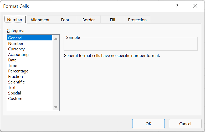Number tab - This is discussed in detail in the Formatting Numbers section.
Alignment tab - Text on the left, numbers on the right.
Font tab - Font, Font style and colour.
Border tab - Borders can be used to separate and define different sections on your worksheet. You can specify different thicknesses and colours.
Patterns tab - Using shading and patterns can make your data dramatically easier to read.
Protection tab - This allows you to lock and prevent users from either changing values or viewing formulas. This is discussed in detail in the Protection section.

Formatting Individual Characters

If you select a cell any formatting will be applied to the whole cell and all its contents.
You can apply formatting to cells, ranges and even Font formatting to individual characters within cells.
To format characters within a cell, double click the cell (to enter edit mode). Highlight the characters you want to format. You will only be able to use the formatting options from the Font tab.
You can select individual characters or words and apply specific formatting.

Formatting as you type

It is possible to have some formatting applied automatically when you enter data although this is only applicable to numeric data.
This type of formatting is possible by using custom number formats.
When you enter numeric characters that represent one of the number formats that Excel recognises, the format is applied automatically.
This is discussed in more detail on the Automatic Formatting page.

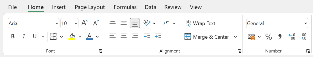
Home Tab

Allows you to alter the appearance and alignment of the data on a worksheet.

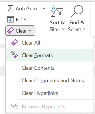
Removing the Formats

You can quickly remove all the formatting associated with a range of cells by selecting the cells. and selecting (Clear > Clear Formats).
To quickly remove just the values, choose (Clear > Clear Contents).
To clear both contents and formats, choose (Clear > Clear All).

Using the CELL() function

This function should help you to determine whether a cell has been formatted as Text or if an apostrophe has been added to the start of the value.

A1 - contains a cell formatted as Text
A2 - contains a prefix

Cell("format",A1) = G - this means it has the general number format ??
Cell("prefix",A2) = ' - meaning the number has been prefixed - although this returns Nothing when the cell is formatted as Text
Cell("prefix",A1) = Nothing
Cell("type") = ?? - returns "v" when the cell contains more that 255 characters

Using the TYPE() function

Merged Cells

To quickly create duplicate merged cells, merge your first cells and then drag the fill handle to create the additional merged cells.
To select cells in a range excluding one value. Select the whole column range. Hold down Ctrl and select the cell of the value you want to exclude. Press (Ctrl + Shift + " | "). If your data is in rows then press (Ctrl + Shift + " \ ").

Double click on the paint brush (located on the Formatting toolbar) to copy a format to a selection of non-contiguous cells. Single click it afterwards to cancel.
You can create automatic list numbering next to cells that contain data with the following formula ("=IF(B1<>"",COUNTA($b$b1:b1)&".","")".

Using the "Extended Formats and Formulas" options Excel will now automatically format a new item added to a list. There must be three of the preceding five rows with the same format. This feature also copies down a formula if the preceding rows contain the same formula.

Smart Tag

Excel 2002 has a new feature associated with the Paste operation.
This is called a smart tag, click it to display the Smart Tag.
It offers several options regarding how to format the cell.
(Tools > Options)(Error Checking tab, "Enable background error checking")
Can we switch this off ???

Other

Numerical values by default are left aligned, however you can use the text alignment prefix characters to change this. Apostrophe(') left aligns. Double quotation marks (") right aligns. Caret (^) centre aligns and a Backslash (\) repeats the characters across the cell.
If you are using text alignment prefix characters to align text then the Caret and Double quotation will only work if you have the following selected (Tools > Options)(Transition tab, "Transition Navigation Keys").
Every time you use a text alignment prefix character on a numerical value a small flag will appear in the upper left corner, indicating a potential problem. If this is intentional, just choose "Ignore Error" from the smart tag menu.
You can suppress the display of positive, negative or zero value by creating a custom number format in which the appropriate section is left blank.
You can format a number as text by prefixing it with an apostrophe (') or entering it as formula surrounded by double quotes.
If you want to avoid using pennies in your prices and your product is priced at $4.42, use the formula =CEILING(4.42,0.05) to round prices up to the nearest nickel.
Numbers in Microsoft Excel can never have more than 15 significant digits, but decimals can be as large as 127.
Any cells that are formatted as percentages are automatically multiplied by 100 so remember to enter them as decimals.
Sometimes when numbers are imported or copied into Excel they are sometimes converted to text

A quick way to convert numbers that are formatted as text to numbers is to multiple them by 1. An alternative is to use the VALUE() function and then copy this down the range
Replacing all "=" with "+" will have the same effect as re-calculating all the formulas in the selection

If a cell is displaying a formula as opposed to the value it could be that the cell is formatted as text.
If you enter a plus sign before a numerical value, then this plus sign is ignored.
If you enter a negative sign before a numerical value, then this is treated as a negative number.
If you see the letter "E" or "e" in a numerical value then this is to denote the exponent and represents "10 to the power" (i.e. 1E7 = 10,000,000).
If you use a forward slash in a numerical value but the entry is not a valid date then this will be interpreted as a fraction (e.g. 5 3/4 = 5.75) (e.g. 1/2 = January 2).
To display a number format that displays millions without showing the 6 zeros use the custom format "0,,".
To quickly remove all formats from a range of cells select (Ctrl + Shift + "~").
To quickly reset the number formats for a selection, press (Ctrl + Shift + "~").
To create a text entry that consists entirely of numbers, you can precede the entry with a text alignment prefix character, typically an apostrophe. (e.g. '123).
You can use a number format to change the colour of your cells. (e.g. "[Blue]$#,#0.00_);(£0.00)").
If you enter a numerical value with a percentage sign then Excel will automatically apply the percentage number format "0.0%". This is equivalent to dividing by 100.
Numbers that are entered in brackets are treated as negative numbers.
To make sure that your fractions are never interpreted as dates precede the fraction with a 0 followed by a space. Excel will use the Fraction number format.

If you enter a dollar sign before any numerical value then Excel will automatically apply the currency number format "-$1,234.10".

A numerical value in a cell will only maintain precision up to a maximum of 15 digits. Excel will convert any digits after the first 15 to zero.
Any numerical value that is too long for the width of the cell is automatically converted to scientific notation, i.e. exponent.
It is important to remember that the number that is "displayed" in a cell is not necessarily the same as the "underlying" value that will appear in the formula bar. The number that is displayed depends on the number formatting and the width of the cell.
You can enter a numerical value as text into a cell by enclosing it in double speech marks (e.g. ="00112233").

Important

If you are going to format your numerical data, try and avoid using red as this colour is normally associated with negative values.
When you copy or cut a cell, the formatting applied to that cell is also copied.
A cell that has been formatted will remain formatted until the formatting is either removed or a different format is applied.
You can toggle bold on the current selection by using the shortcut key (Ctrl + B).
You can toggle italics on the current selection by using the shortcut key (Ctrl + I).
The Format Painter lets you copy the formatting attributes from cells you have previously formatted to other cells.