GETPIVOTDATA(data_field, pivot_table [,field1] [,item1] [..]))
The GETPIVOTDATA function returns the data obtained from a pivot table.
This worksheet function can be used to retrieve specific values from a pivot table.
It is possible to use a regular formula that links to the cell reference inside the pivot table but this is dangerous as the pivot table may be filtered to display different data.
In order to use this function effectively you have to ensure that your pivot table as the appropriate descriptive information.
You must pass to the function the descriptive name of the column you want to retrieve and the corresponding row items to match.
Simple Example
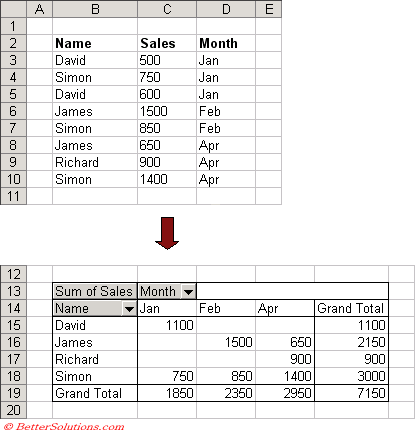
Lets consider a very simple table:
 |
The GETPIVOTDATA() function has two required arguments and can have up to 14 pairs of optional arguments.
For this example we are assuming that the worksheet functions are on the same worksheet as the pivot table.
If the pivot table is located on another worksheet then the worksheet name must also be included in the "pivot_table" argument.
Returning the total from a single field
This example returns the total for the values in the "Sales" column of the table.
The "data_field" is "Sales" as we want to return all the values in the Sales column or field of the table.
The "pivot_table" can be any cell within the table, in this case B13.
| =GETPIVOTDATA("Sales",B13) = 7150 |
Returning the value matching two fields
This example returns the total "Sales" for the values that have a month of "Jan".
The "data_field" is "Sales" as we want to return all the values in the Sales column of the table.
The "pivot_table" can be any cell within the table, in this case B13.
We also want to filter on the "Month" field.
Filtering out just the "Jan" months.
| =GETPIVOTDATA("Sales",B13,"Month","Jan") = 1850 |
Returning a specific value matching all three fields
This example returns a specific item in the pivot table. This returns Richard's sales contribution for the month of "Apr".
The "data_field" is "Sales" as we want to return all the values in the Sales column of the table.
The "pivot_table" can be any cell within the table, in this case B13.
We also want to filter on the "Month" field.
Filtering out just the "Apr" months.
We also want to filter on the "Name" field.
Filtering out just the "Richard" months.
| =GETPIVOTDATA("Sales",B13,"Month","Apr","Name","Richard") = 900 |
Important
Remember that is the pivot table is located on another worksheet then the worksheet name must be included in the "pivot_table" argument.
© 2024 Better Solutions Limited. All Rights Reserved. © 2024 Better Solutions Limited TopPrevNext