Pivot Table Wizard

Removed in 2007
You can display the Pivot Table wizard by selecting (Data > PivotTable and PivotChart Report).

Pivot Table Report - Starts the Pivot Table and Pivot Chart Wizard, which guides you through creating or modifying a PivotTable or PivotChart report.

There are three steps allowing you to change the type of report, the data to use and the location of your pivot table.
The pivot table wizard will take you through the three stages.
Step 1 - Type of Report - Lets you choose where the data is coming from either an Excel list or database, external source, consolidation of ranges or even another pivot table.
Step 2 - Source Data - Lets you select the cells and define the range to use for the source data. If the insertion point is anywhere within the Excel list or database then the whole block of cells will be selected automatically.
Step 3 - Location - Lets you decide whether to display the pivot table report on a new worksheet or on the existing worksheet
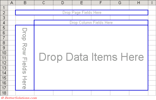
Step 3b - Layout - This is not a separate step in the Wizard as it can either be done before or after the pivot table has been created. This lets you determine the exact layout of the report by dragging the fields onto a pivot table diagram.

Type of Report

Highlight any cell within the data and select (Data > PivotTable and PivotChart Wizard).
Your data must contain column headings as these will be automatically used for the pivot table fields.

Creating just a pivot table with an Excel list is the default option so press Next.
Note that the graphics down the left hand side change to confirm your selection.

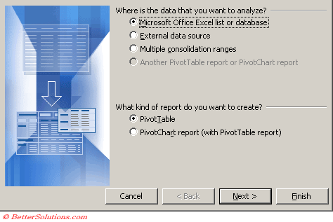Microsoft Excel list or database - You data table must have unique column labels at the top of each column.
External data source - Includes Access databases and other Excel workbooks.
Multiple consolidation ranges - Multiple ranges containing similar data.
Another PivotTable or PivotChart -

Source Data

If you are using an Excel list and you have selected a cell within the list before invoking the wizard then the continuous range of cells will be selected.
If you select a single cell for the source data before displaying the Wizard the current region will be automatically selected. You can change this in step 3 of the Wizard ??
All the data should be highlighted so press Next.

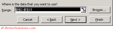Excel will automatically select the range of cells in the continuous range.
It is possible to change the source data range after the pivot table has been created.
Holding down the Shift key and pressing on the lower right cell will extend the data source to include that cell.
You can also insert rows into the data source and the data will automatically be included the next time the pivot table is refreshed.

Location

Decide whether you want to insert the pivot table onto a new worksheet or the existing worksheet.
Before clicking on the Finish button you can select Layout button to define the table layout of your pivot table.

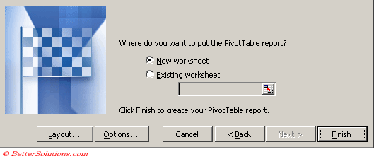New worksheet - A new worksheet will be inserted before the active sheet containing your pivot table report. This is the default.
Existing worksheet -
Layout - You can always changes these at any point after the pivot table has been created.
Options - Displays the (PivotTable > Table Options) dialog box.

Layout

After you have completed the steps the pivot table field list will be displayed to let you change how the table is organised.

Final PivotTable

The following pivot table summarising your data will be displayed.

Important

You should also enter a name for the pivot table, the default will be PivotTable1, PivotTable2, etc
If you assign the named range "Database" to your cell range it will be recognised automatically.
If possible it is always better to base a new pivot table on an existing one as it will use the same memory cache for both tables.