Comparing

Comparing Two Ranges

The quickest way to compare two ranges of data is to use Conditional Formatting.
Depending on exactly what you want to compare will depend on which formula you use.
=NOT(B3=F3) - will compare the contents of every cell relative to its position in the table.
=COUNTIF(F3:H14,B3)=0 - will compare occurrences in each column.
=User Defined Function - will compare whole rows of data in a table.
To make the formulas a little easier to understand select the first range of data, in this case "B3:D14" and assign it the named range "Table1".
Do the same for the second range of data, in this case "F3:H14" and assign it the named range "Table2".
When comparing cells, numbers formatted as text is always greater than the equivalent number.

Comparing Every Relative Cell

Conditional formatting can be used to compare the contents of every cell in two tables.

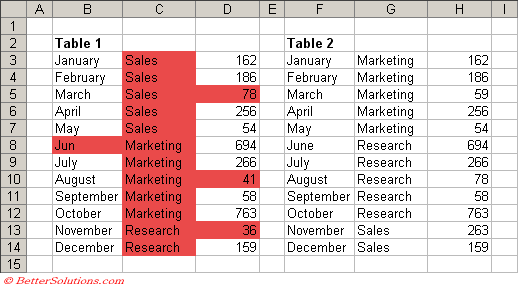Select cells "B3:D14" and select (Format > Conditional Formatting) to display the Conditional Formatting dialog box.
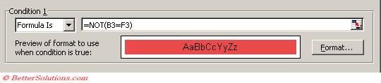
Select the "Formula is" in the first drop-down list and enter the formula "=NOT(B3=F3)".
Click the Format button to apply your specific formatting, in this case we are just applying a red background.

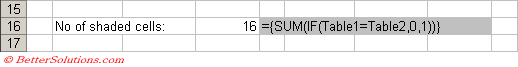
You can quickly get the total number of cells that are different by using the following Array Formula.
This formula must be entered by pressing (Ctrl + Shift + Enter).

Comparing Occurrences

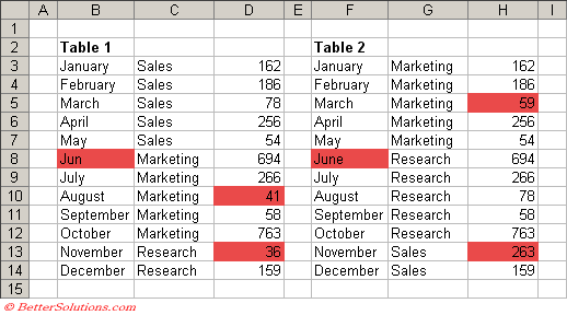
Conditional formatting can be used in conjunction with the COUNTIF function to identify items that do not occur in their respective columns.
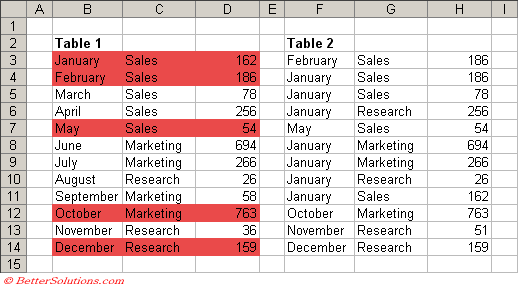
Notice that none of the cells in the middle column are shaded since all these items occur in both tables.
Notice also that the number 78 in cell "D5" is not shaded, this is because there is an occurrence in cell "H10".
Notice also that the number 78 in cell "H10" is not shaded, this is because there is an occurrence in cell "D5".

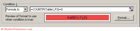
Select (Format > Conditional Formatting) to display the Conditional Formatting dialog box.
Select the "Formula is" in the first drop-down list and enter the formula "=COUNTIF(Table2,B3)=0".
Click the Format button to apply your specific formatting, in this case we are just applying a red background.

Select (Format > Conditional Formatting) to display the Conditional Formatting dialog box.
Select the "Formula is" in the first drop-down list and enter the formula "=COUNTIF(Table1,F3)=0".
Click the Format button to apply your specific formatting, in this case we are just applying a red background.

The cell reference in the COUNTIF function should always be the upper left cell of the current selection.

Comparing Rows

Conditional formatting can be used in conjunction with a user defined function to identify which rows appear in a table.

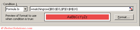
Select cells "B3:D14" and select (Format > Conditional Formatting) to display the Conditional Formatting dialog box.
Select the "Formula is" in the first drop-down list and enter the formula "=matchingrow($B3:$D3,$F$3:$H$14)".
This formula will highlight all the rows that do occur in the table.
If you want to highlight the rows that do not appear then you can change the formula to "=matchingrow($B3:$D3,$F$3:$H$14)=0".
Click the Format button to apply your specific formatting, in this case we are just applying a red background.

The function defined below allows you to pass in a single row of cells and a table of cells.
The value returned will be the row number of the first occurrence or zero if the row does not exist.

Public Function MatchingRow(ByVal rgeRowToMatch As Range, _ 
                            ByVal rgeTableOfData As Range) As Long 
Dim lcheckrowno As Long 
Dim lcurrentrowno As Long 
   Call Application.Volatile(True) 
   For lcheckrowno = rgeTableOfData.Row To (rgeTableOfData.Row + rgeTableOfData.Rows.Count - 1) 
      lcurrentrowno = lcheckrowno - rgeTableOfData.Row 
      If rgeRowToMatch.Cells(1).Value = rgeTableOfData.Cells(1).Offset(lcurrentrowno, 0).Value Then 
         If ColumnsMatching(rgeRowToMatch, rgeTableOfData, lcurrentrowno, 2, rgeRowToMatch.Cells.Count) = True Then 
            MatchingRow = lcheckrowno 
            Exit Function 
         End If 
      End If 
   Next lcheckrowno 
End Function 

Public Function ColumnsMatching(ByVal rgeRowToMatch As Range, _ 
                                ByVal rgeTableOfData As Range, _ 
                                ByVal lRowNo As Long, _ 
                                ByVal iColNo As Integer, _ 
                                ByVal iNoOfColumns As Integer) As Boolean 
Dim icolumnno As Integer 
Dim iallmatch As Integer 
   iallmatch = 0 
   For icolumnno = iColNo To iNoOfColumns 
      If rgeRowToMatch.Cells(icolumnno).Value <> rgeTableOfData.Cells(1).Offset(lRowNo, icolumnno - 1).Value Then 
         iallmatch = iallmatch + 1 
      End If 
   Next icolumnno 
   If iallmatch = 0 Then ColumnsMatching = True 
   If iallmatch > 0 Then ColumnsMatching = False 
End Function