Multiple Conditions

You can include up to three different conditions on any cell or range of cells.
For example your three conditions might be:
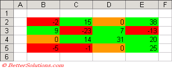
0) If the number < 0 then shade the cell red.
1) If the number = 0 then shade the cell orange.
2) If the number > 0 then shade the cell green.

First Condition

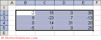
We are going to apply conditional formatting to the range of cells "B2:E5" and we are going to shade all the cells identifying whether they are negative, zero or positive.
Select the range of cells you want to apply the conditional formatting to, in this case cells "B2:E5".

Select (Format > Conditional Formatting) to display the Conditional Formatting dialog box.
Select "Cell Value Is" in the first drop-down box and "less than" in the second dialog box.
Enter the constant value 0 in the third box.
Click the Format button to apply your specific formatting, in this case we are just applying a red background.

Second Condition

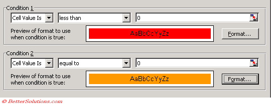
You can add another condition by pressing the "Add" button.
Select "Cell Value Is" in the first drop-down box and "equal to" in the second dialog box.
Enter the constant value 0 in the third box.
Click the Format button to apply your specific formatting, in this case we are just applying a orange background.

Third Condition

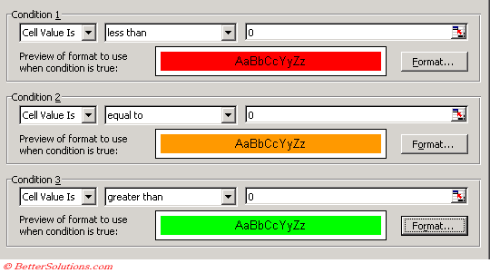
You can add another condition by pressing the "Add" button.
Select "Cell Value Is" in the first drop-down box and "greater than" in the second dialog box.
Enter the constant value 0 in the third box.
Click the Format button to apply your specific formatting, in this case we are just applying a green background.

Press OK to apply your conditional formatting.

Important

If you specify more than one condition it is the formatting associated with the first condition which is true, which will be applied to the cell (or range of cells).