Pivot Tables

A Pivot table allows you to "interactively" aggregate your data and is a great way to generate a dynamic summary report.
The term pivot refers to being able to change the position of the fields and to being able to transpose the rows and columns of your table.
The more data you have to analyse then the more appropriate it is to use a pivot table.
Pivot Tables are designed for dynamic viewing of database data (either contained within Excel or from an external source).
Pivot Tables are always linked to the data they are derived from.
When a Pivot table is created Excel builds a special memory cache containing your data. This allows you to change and recalculate your data.
The data you will want to analyse will normally be numerical values, although it is possible to also use text values as well.

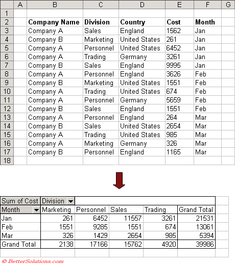Looking at the Excel list it is hard to identify how much is being spent a month on each division.
The pivot table below summarises this Excel list and makes it much easier to understand.

Allow you to structure, summarise and compare data.
They are especially useful for:
Subtotalling and aggregating
Summarising based on categories
Collapsing data and drilling down
Filtering, sorting and formatting

In a PivotTable each column becomes a field

Advantages of using a Pivot Table

To help identify relationships within your data that would otherwise be hard to see due too the quantity of data.
To aggregate and summarise a large quantity of data into a smaller more condensed table.
To organise your data into a format that would be easy to chart.
Pivot tables are dynamic allowing you to change the appearance instantly and because the table is linked to your original data it can be refreshed extremely quickly.
You can quickly include and exclude individual fields from your summary table.
Data can be grouped together using outlines and individual rows and columns can be hidden.

Different Types of Calculation

Summary Function - SUM, COUNT, AVERAGE, MIN, MAX, PRODICT, STDDEV, STDDEVP, VAR, VARP
Custom Calculations - Percentages, Running Totals, Index Values, Differences. Once the report has used a summary function an additional calculation is required
Formula - Lets you perform calculations against data in other fields and return the results to a new Calculated Field in the Values area

Pivot Charts

You can create charts that are directly linked to your pivot table results.
It is even possible to change the data layout by adjusting the chart.

Potential Problems

If someone adds or deletes a column in the original source data, the pivottable cannot be refreshed and displays an error.

You can use a pivot table to link to a range of data on another sheet and display it in a different order.
A pivot table is extremely useful when you have lots of changing rows, or blank rows , when the number of rows changes frequently.

Showing and Hiding Data

You can hide an inner field by double clicking on its outer field.
Double click the outer field heading to display the inner field.
Alternatively you can show and hide fields by selecting the corresponding button on the PivotTable toolbar.

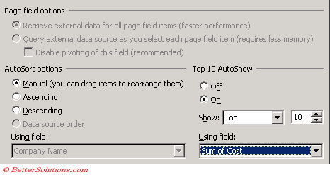
AutoShow

You can use the AutoShow feature to display only a certain number of items in a field based on values in the data area of your table.
Choose the field in the pivot table and select (PivotTable > Field Settings)
Select Advanced.

Empty Cells and Cells containing Errors

By default cells that do not contain any numbers in the data area are left blank.
It is possible to display a value or a text entry in any empty cells.

It is possible to use formulas to calculate additional fields in your pivot table, and it is possible that this formula might return an error.
It is possible to display an empty cell, value or a text entry in any cells that contain errors.

Using a subset of Data

If you only want to use part of a list then you must use the advanced filter to filter the relevant data to another location on the worksheet.
Specify the location of your source data

Moving a Pivot Table

Once a pivot table has been created it can be easily moved.
It can be moved either by using the wizard or by cutting and pasting the cell range that contains the pivot table.
Select any cell in the table and select (Data > PivotTable and PivotChart Report). Specify a new cell address on the existing worksheet.

Pivot Table Restrictions

You cannot create a pivot table that contains more than 8000 total items.
You cannot create a pivot table that contains more than 256 fields in the Data Area.

Multiple Consolidation Ranges Example

To switch from one summary function to another select an item in the data area of your pivot table, click the field settings button and then choose from the list that appears in the Pivot Table field dialog box.

Grouping on a particular field can be very useful if you want summarize data over a range of values -- Right-click the field label and choose Group and Outline | Group...
Blank rows in the data set will prevent you from using Grouping in your Pivot Table

Use pivot tables as an alternative to linking workbooks using formulas
SS good examples

Important

Pivot Tables work well when you have large amounts of data to analyse.
The simplest type of pivot table is just an aggregate of a single column which could be used to show the number of occurrences of each item in a list.
If you are using a data list on a worksheet then all your columns must have labels as these will be used as the field names.
You must remove any automatic totals or subtotals from your list before the pivot table as the pivot table report will create any necessary total automatically.
Referring to a named range on a different worksheet in the same workbook works. Referring to a named range in a different workbook doesn't work.
The entire list will be used to generate the pivot table and any hidden rows will be included.