Displaying Multiple Dependent Drop-Down Lists

In this example we are going to create three drop-down lists.
Depending on the value selected in the first drop-down list will determine what values are displayed in the second.
And then depending what value is selected in the second drop-down list will determine what values are displayed in the third.

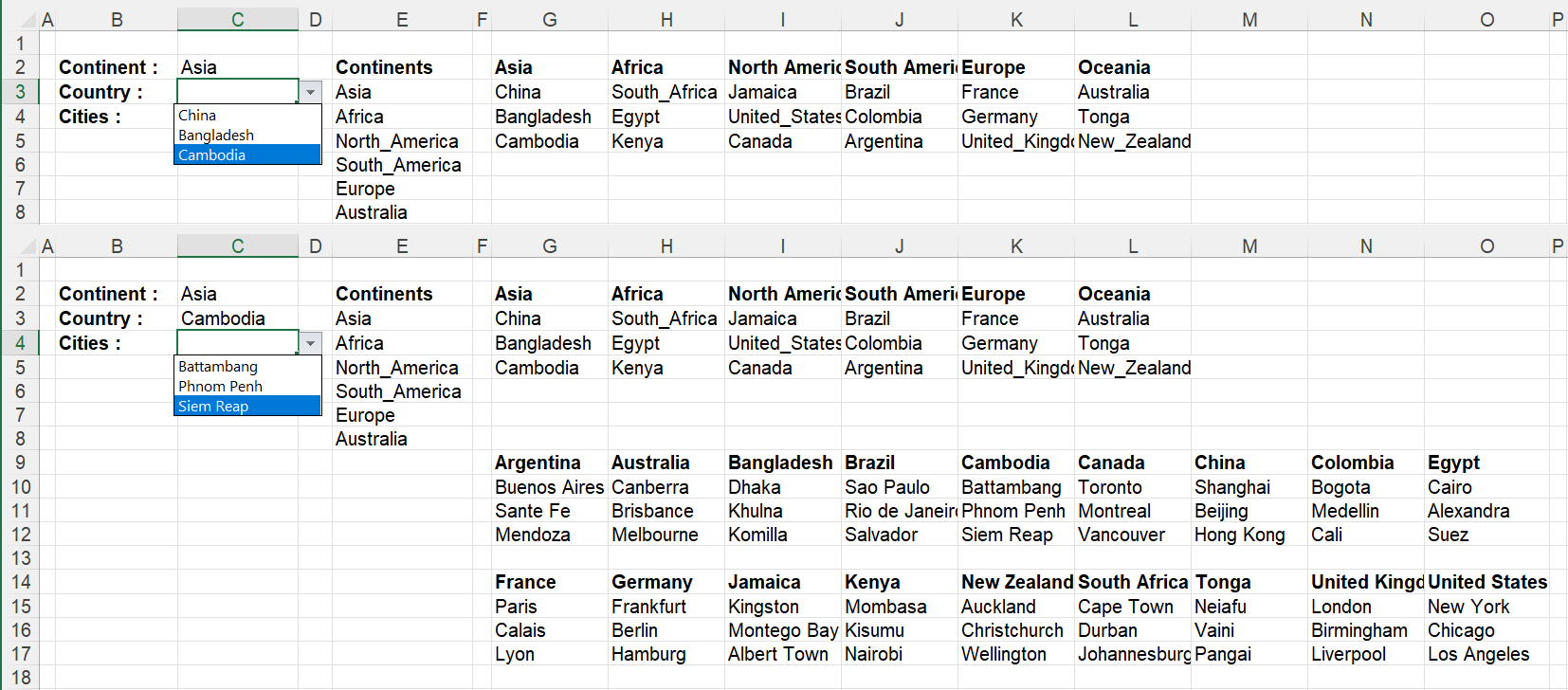
Create a table with all the corresponding values.
Our first category is going to be Continents E3:E8. Each continent is going to have three countries
Our second category is going to be Countries and each country is going to have three cities.

Create the Named Ranges (for the Continents)

Highlight the cells "E3:E8". Select Formulas tab, Define Name and type the name "Continents".
Highlight the cells "G3:G5". Select Formulas tab, Define Name and type the name "Asia".
Highlight the cells "H3:H5". Select Formulas tab, Define Name and type the name "Africa".
Highlight the cells "I3:I5". Select Formulas tab, Define Name and type the name "North_America"
Highlight the cells "J3:J5". Select Formulas tab, Define Name and type the name "South_America".
Highlight the cells "K3:K5". Select Formulas tab, Define Name and type the name "Europe".
Highlight the cells "L3:L5", Select Formulas tab, Define Name and type the name "Oceania".

Create the Named Ranges (for the Countries)

Highlight the cells "G10:G12". Select Formulas tab, Define Name and type the name "Argentina".
Highlight the cells "H10:H12", Select Formulas tab, Define Name and type the name "Australia".
Repeat the same process for the following 16 countries.

Enter the Criteria for the Continent Drop-Down List

Select the cell you want the first drop-down list to appear in, in this case cell "C2".
Select Data tab, Data Validation, Settings tab.
In the Allow drop-down box select "List".
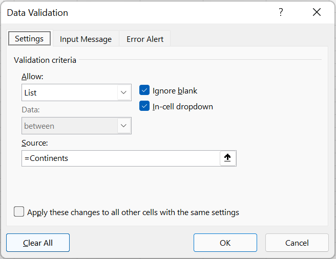
In the Source box enter the formula "=Continents" to refer to the named range that you created earlier.

Enter the Criteria for the Country Drop-Down List

Select the cell you want the first drop-down list to appear in, in this case cell "C3".
Select Data tab, Data Validation, Settings tab.
In the Allow drop-down box select "List".
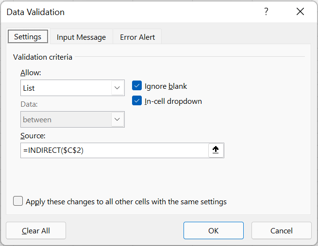
In the Source box enter the formula "=INDIRECT($C$2)" to refer to the named range that you created earlier.

Enter the Criteria for the City Drop-Down List

Select the cell you want the first drop-down list to appear in, in this case cell "C4".
Select Data tab, Data Validation, Settings tab.
In the Allow drop-down box select "List".
In the Source box enter the formula "=INDIRECT($C$3)" to refer to the named range that you created earlier.

Displaying the Countries and Cities in Asia

Select cells "C2:C4" and delete the contents.
Select cell "C2" and choose "Asia" in the drop-down.
Select cell "C3" and choose "Cambodia" in the drop-down.
Select cell "C4" and choose "Siem Reap" in the drop-down.