Copying

Copying the Results to Another Location

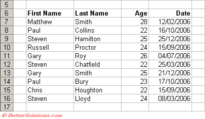
Instead of filtering the list in-place you could copy the results to another location on the same worksheet.
It is not possible to copy the results to another worksheet or workbook.
The criteria can be on a different worksheet but the results can only be copied to the same worksheet.

More Complicated Formulas

The example we are going to use here will use a more complicated formula in its criteria.
When you use more complicated formulas the criteria heading used must not be the same as any of the table column headings.
In this case we have used the heading "Criteria" instead of "First Name".
If you use the heading "First Name" only the heading appears in the "Copy to location".
Alternatively you could leave it blank but even when left blank the criteria still needs to include both cells.

Any formulas you do use have to return either TRUE or FALSE.
You will also need to include the necessary absolute and relative references (in this case cell "B7").
A particular row is only included when the formula returns TRUE for that particular line.

Creating the Formula

In this example we are going to extract all the names that appear more than once in the "First Name" column.
The function that can help us with this task is the COUNTIF function.
This function returns the number of cells with a value that satisfies a condition.

Absolute and Relative References

When you are using formulas for your conditions it is important to know when to use absolute and when to use relative references.
Absolute references should be used for any cell ranges that you want to remain fixed within the formula.
Relative references should be used for any cell ranges that are relative to the row that is being analysed at the time.
For example we want to be able to determine if an item appears more than once in a particular column.
For this we will use an absolute cell reference for "B7:E16" but a relative cell reference for the cell range passed as the criteria to the COUNTIF function.

Enter the Condition

Enter the following formula in cell "B3" above the table.

Select a cell inside the table, for example cell "C7" and select (Data > Filter > Advanced Filter).
Check that the "List range" references the whole table.
In the "Criteria range" textbox select the cells "B2:B3".
Select the option "Copy to another location".
In the "Copy to" textbox select cell "B18" (this is the first cell where you want the results to start).
Check you have entered all the information correctly and press OK.

Extract - Worksheet Level Named Range

When you specify a "Copy To" range Excel will automatically assign the named range "Extract" to the "Copy To" cell range.
This named range can be used to quickly select the extacted range.
Select (Edit > GoTo) and type in "Extract" and press OK.
This probably wont be much use though because in this case it only refers to the first cell, i.e. cell "B18".

Important

Criteria on the same line (different columns) are joined by AND and criteria on a new line (same column) are joined by "OR".
You can quickly display all the rows from a filtered list by selecting (Data > Filter > Show All).