Filtering

AutoFilter is the quickest and easiest way to filter a table (or list) of data.
When we use the word "filter" we are just temporarily hiding the rows that we do not want to see.
This feature displays drop-down lists at the top of each column and allows the user to select unique values within each column in order to filter the data accordingly.
These drop-down lists can then be used either individually or in combinations to filter the data within your table.
When a table is "filtered" the rows that do not match the value you have chosen from the drop down list are hidden.

Filtering Restrictions

There are a three very important restrictions you need to be aware of:
0) Your table must contain column labels because any filter is not applied to the first row.
1) You can only have one AutoFilter per worksheet.
This means that you cannot have multiple filtered tables on the same worksheet.
0) An AutoFilter drop-down list will only show 1000 entries, and that setting cannot be changed.
If your column has more than 1000 "unique" items you might have to use the "custom" option from the drop-down list to enter your filter criteria. For more details, please refer to the AutoFilter - Custom page.

Applying the Filtering

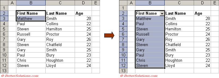
You can apply auto filtering to a table of data by selecting any cell in the table (in this case "B5") and selecting (Data > Filter > AutoFilter).
Drop-down menus will then appear to the right of each column heading in the first row of the table.
Clicking the arrow on the drop-down list will display all the unique items in that column (in alphabetical order).

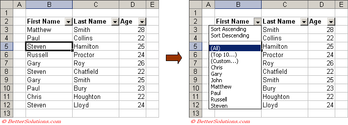The options "All", "Top 10" and "Custom" will appear automatically.
The "Sort Ascending" and "Sort Descending" options will also appear automatically although these were only added in 2003.
If a particular column contains any empty cells then "Blanks" and "NonBlanks" will also appear automatically at the bottom of the list.

One Column Filtering

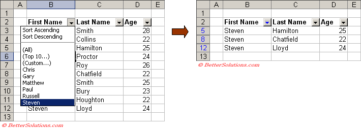
It is then extremely easy to filter the table so it only displays unique items from a particular column.
This is very useful when you have large table containing hundreds or maybe thousands of rows.
In this example we select "Steven" in the first drop-down list.
Any column that has a filter currently applied has its drop-down arrow changed to blue.
The row numbers of the filtered table also have been changed to blue. Again this is to remind you that the rows have been filtered.

All - To display all the rows in the table after a filter has been applied, select "(All)" in the drop-down list that contains a filter. Alternatively you can select (Data > Filter > Show All).
Top 10 - This is discussed in detail later on. For more details, please refer to the AutoFilter - Top 10 page.
Custom - This is discussed in detail later on. For more details, please refer to the AutoFilter - Custom page.

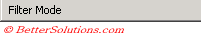
The bottom left corner of the status bar is used to indicate if a Filter has been applied to a table on the active worksheet.

Several Column Filtering

It is possible to refine your filtering even further by using drop-down lists in the additional columns.
Notice that when a table has been filtered by one column the other drop-down lists only display items from the "filtered" table.
You can filter by another criteria by selecting another item in one of the other drop-down list boxes.
Select the third drop-down list and select "22".
This will filter the list even more to only display rows that have 22 in column D.

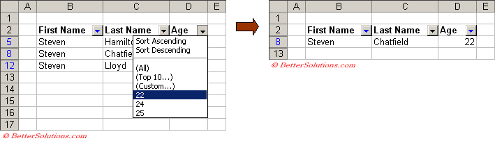The rows that do not have the number 22 in column "D" have been hidden.

Using Filtering (specific columns)

If you only want the drop-down lists to appear in certain columns, select only these column labels before selecting (Data > Filter > AutoFilter).
Note that the columns must be next to each other.
If you only want the drop-down list to appear in one column, select the first two cells in this column.
In this example we only want a filter drop-down list displayed for the first column so we select cells "B2" and "B3".

Removing the Filtering

To remove an AutoFilter altogether select (Data > Filter > AutoFilter) to remove the check box.
To display all the rows in the table after a filter has been applied, select "(All)" in the drop-down list that contains a filter. Alternatively you can select (Data > Filter > Show All).
Need a quick way to toggle/remove all filters ?

Important

If you select more than one cell within a table before applying the AutoFilter only the selected cells will have the drop-down lists added and not the whole table. Unlike the Sort command there is no prompt or warning.
You can apply AutoFilter to a selection of columns in your data table by selecting the column labels first before selecting (Data > Filter > AutoFilter).
You can only have one AutoFilter per worksheet, which means that you cannot have multiple filters below each other ??
Once you have applied a filter, either using AutoFilter or Advanced Filter the table of data is given the named range "_filterdatabase". This name does not appear in the named range dialog box but typing this named range into the (Edit > GoTo) dialog box will select the whole table.