Advanced Filter

Advanced Filter allows you to filter using more than two criteria and also allows you to use formulas in your conditions.
Advanced Filter also allows you to obtain a list of unique items and/or copy the matching rows to another location.
The conditions which are used by the advanced filter have to be specified in separate cells to the actual table (typically above the table).

The specification of the conditions is very similar to that of the Database Functions.

Criteria Range - Rules

The criteria range must be in a cell range that is separate from your table of data. It must be separated by at least one blank row or column.
The criteria range must consist of at least two rows, containing the column heading and the criteria.
You can include as many criteria as you like.
Any blank cells in your criteria range will mean that ANY values can be accepted for this column.
The criteria can be on a different worksheet.

Greater Than 23 AND Less Than 26

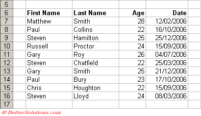
The first thing you must do is make sure that your table is setup correctly and that you have several blank rows above your table.
The blank rows at the top will be used to specify the Advanced Filter conditions.
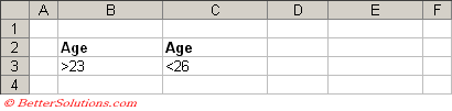
In this example we are going to use the AND operator with two conditions on the "Age" column.
When you want to specify an AND operation you must place the conditions in separate columns.
The first condition is that "Age" is greater than 23, so this is defined in cells "B2:B3".
The second condition is that "Age" is less than 26, so this is defined in cells "C2:C3".

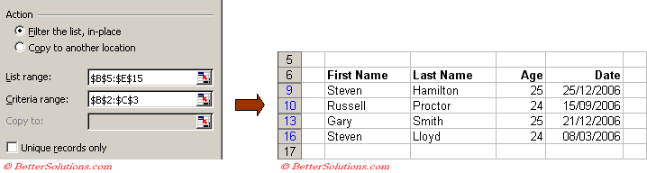
Select a cell inside the table, for example cell "C7" and select (Data > Filter > Advanced Filter).
Check that the "List range" references the whole table.
In the "Criteria range" textbox select the cells "B2:C3" and press OK.

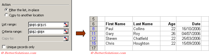
Either 22 OR 26

In this example we are going to use the OR operator with two conditions on the "Age" column.
When you want to specify an OR operation you must place the conditions in the same column.
The first condition is that "Age" is 22, so this is defined in cells "B2:B3".
The second condition is that "Age" is 26, so this is defined in cell "B4".

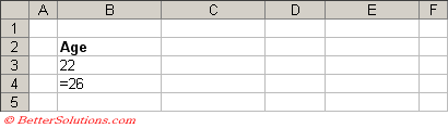Including the equal sign (=) is optional.
Select a cell inside the table, for example cell "C7" and select (Data > Filter > Advanced Filter).
Check that the "List range" references the whole table.
In the "Criteria range" textbox select the cells "B2:B4" and press OK.

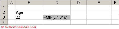
Include Formulas In Your Criteria

It is even possible to use formulas to provide the conditions for your filter.
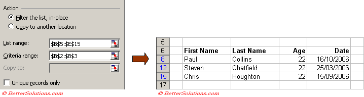
In this exampe we are going to only show rows where the "Age" is the smallest in the table.
The first thing we need to do is to obtain the smallest age from the table.
This can be done using the MIN function.
Enter the formula "=MIN(D7:D16)" into cell "B3" to form the necessary value for the criteria.

Criteria - Worksheet Level Named Range

After you have used the Advanced Filter the cell range which you used to define your conditions will be given the named range "Criteria".
This named range is automatically assigned when your criteria is on the same worksheet as the actual table.
This named range can be used to quickly select the extacted range.
Select (Edit > GoTo) and type in "Extract" and press OK.

Important

AutoFilter allows you to filter using a maximum of two criteria.
Criteria on the same line (different columns) are joined by AND and criteria on a new line (same column) are joined by "OR".
You can quickly display all the rows from a filtered list by selecting (Data > Filter > Show All).
You can access named ranges from (Insert > Name > Define). For more details on named ranges see the Named Ranges section.