with Drop-Down

Highlight the cells

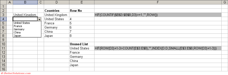
This example shows you how to prevent a user from selecting the same value more than once from a drop-down list.
Basically once the entry has been selected the item is automatically removed from the other drop-down lists.

This solution is quite advanced and requires a good understanding of both functions and formulas.

Find the correct formula

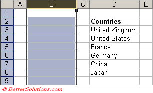
First create a list of all the items you want to appear in the drop-down list.
In this example we have entered these as a list in column "D" in cells "D3:D8".
Next you need to add a formula that can indicate if the entry has already been selected.
The COUNTIF function returns the number of non blank cells with a value that satisfies a condition.
The ROW function returns the row number of the cell containing the formula.
In this example these formulas are going to be entered in column "E" in cells "E3:E8".
=IF(COUNTIF($B$3:$B$8,D3)>=1,"",ROW())

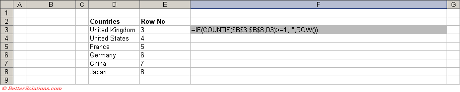If this particular entry already exists in column B the cell will appear blank otherwise, the corresponding row number will be displayed.
Drag this formula down to the cells below ("E4:E8").
Using the formula that we have just entered we need to enter another formula.
This formula will create a list of "unused" items containing only the items that have not already been entered into column "B".
The COUNT function returns the number of numeric values in a list or array of numbers.
The INDEX function returns the value from a list based on an index number.
The SMALL function returns the smallest value in a data set.
The INDIRECT function returns a text string of the contents of a given cell reference.
The ROWS function returns the number of rows in a cell range or reference.
In this example these formulas are going to be entered in column "E" in cells "E11:E16".
=IF(ROW(D3)+1-3>COUNT(E$3:E$8),"",INDEX(D:D,SMALL(E$3:E$8,ROW(D3)+1-3)))

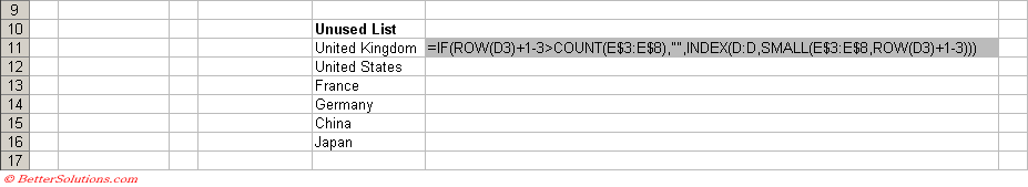The number 3 represents the row of the first item in the list from cell "D3".

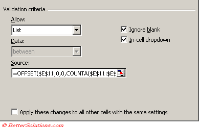
Activate the Data Validation dialog box

Highlight the cells you want to apply the data validation to. In this case the whole of column B.
Press (Data > Validation) to display the Data Validation dialog box and select the Settings tab.
In the "Allow" drop-down box, select "List" (or Custom).
Enter the following formula as the Source:
=OFFSET($E$11,0,0, COUNTA($E$11:$E$16)-COUNTBLANK($E$11:$E$16),1)
For more details on these types of formulas, please refer to the Dynamic Named Ranges page.

Enter some values

Select cell "B3". Notice that the drop-down list displays all six items.
Pick "United Kingdom" from the list and then select "B4".
Notice that only the only five items are now displayed.