Freeze Panes

Freeze panes allow you to freeze the top or left or both on the active worksheet.
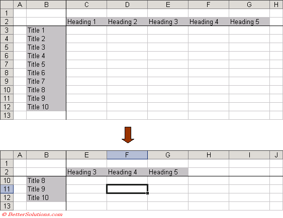
Using freeze panes lets you keep the column headings or row titles visible while while you scroll to other parts of the worksheet
The frames that are not frozen will scroll but will not affect the area that is frozen.
Many large worksheets contain row and column headings to identify the data in tables.
As you scroll the worksheet the headings will often disappear from view.
This can be prevented by taking advantage of the Freeze Panes.

You can freeze the top horizontal pane by clicking the row below where you want the split to appear.
You can freeze the left vertical pane by clicking the column to the right of where you want the split to appear.
You can freeze both the upper and left panes by clicking the cell below and to the right of where you want the split to appear.
(Window > Freeze Panes)
The row and column headings will remain on the screen as you scroll around the worksheet.
You can unfreeze the window at any time by selecting (Window > Unfreeze Panes.

It can be useful to freeze parts of a worksheet to allow you to freely move to other parts of the worksheet.
The most common use for this is when you are scrolling a large table of information and you want to keep the column and row headings visible while you scroll through the whole table.
They may be times when you need to keep multiple rows or multiple columns "frozen" at the top of to the left of your screen.
Excel will use dark lines to indicate when any rows or columns have been frozen.
These frozen rows and columns will remain visible as you scroll through the worksheet.

Adding Freeze Panes

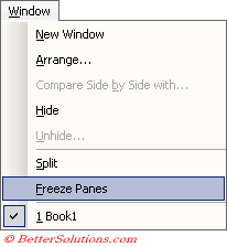If you want to freeze rows at the top of a worksheet as well as columns on the left then select the cell which is to the right of the column you want to freeze and below the row you want to freeze and select (Window > Freeze Pane).
If you want to freeze a row at the top of a worksheet, select the row below the one you want to freeze and select (Window > Freeze Pane).

If you want to freeze rows at the top and columns on the left then select the cell which is to the right of the column you want to freeze and below the row you want to freeze and select (Window > Freeze Pane).

Removing Freeze Panes

Select the worksheet that contains the frozen panes and Select (Window > Unfreeze Panes).
If you want to unfreeze the rows, select the row below the last one that is frozen and select (Window > Unfreeze Panes).

Important

This feature can be used in connection with Split Panes
Excel will freeze all the rows above the row which you select.
Excel will freeze all the columns to the left of the column you select.
Dark lines to indicate when any rows or columns have been frozen.
Freezing panes has no effect on how the worksheet is printed. To control which rows and columns are repeated when printing, please refer to the Page Setup - Sheet Tab page.