Understanding the Pivot Table Layout

A field will basically act as a filter for your data.
For each field that you want to use in order to filter your data, you can specify exactly which items to include.
The page field can only have one field associated with it.
This is not actually part of the wizard steps ?
Changing the layout of the Pivot Table is not an actual step in the Wizard as it can be done either before or after the pivot table report has been created.
1) During the Pivot Table Wizard, pressing the Layout button on Step 3.
2) Using the PivotTable Field List Pane.
3) Dragging the fields once the pivot table has been created.

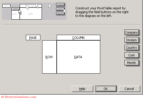
Using the Pivot Table Layout Dialog Box

There are four types of field types,
Page - Filters your view by data in the table by dividing the report into smaller pages allowing to you view one at a time.
Column - This field controls the actual data that is displayed and defines the column headings for your custom report. Any buttons that you drag to the Column area will automatically appear as separate columns.
Row - This field controls the actual data that is displayed and defines the row headings for your custom report. Any buttons that you drag to this area will appear as separate rows.
Data - These fields identify the data to be summarised. If you add more than one field to the data area if your pivot table, then subtotals will be displayed automatically. You can have more than one. There are many different ways that your data can be aggregated. This is discussed on a later page.

All the fields or column headings from your data source will be displayed as field buttons down the right hand side of the dialog box.
These buttons can be dragged to the relevant areas of the table to define the pivot table.
You must always have a field on the data area of your pivot table.

All the field names from the data source are displayed on the right hand side as buttons and can be dragged and dropped on to any of the four areas of the pivot table.

Dragging the Field Buttons

You can use your mouse to drag the field buttons to any of the four locations on the table to define your pivot table.

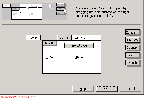For every item that appears in a row field or column field there will be a corresponding row or column added to your pivot table.
When you drag a field to the Data area the Sum function is applied by default.
If the values in that particular field are not numeric, then the COUNT function will be applied by default.
You can summarise the data in a number of different ways and there are several function that can be used. This is discussed in more detail on the Data Area Calculations page later on.
You can include multiple field buttons in each of the four layout locations.
All the data for a particular field can be displayed when it is in the column or row areas of a pivot table.
A pivot table can include several fields in its page area although they are only stored on a single worksheet.
When you use the Page field to filter a large amount of data into separate pages. You can either view all the values or one specific value.
You can place multiple fields on any of the row, column or data areas.
It is possible to change the name of the fields that have supplied to the pivot table.
Just select the field name and type in a different name.
You must remember to always keep all your fields distinct.
Moving a row or column field to the page field lets you "zoom in" on a particular field.
Subtotals and Grand totals will be created automatically by default.

Dragging the fields once the pivot table has been created

To remove a field from the pivot table drag the field to an empty part of the worksheet.
If you want to exclude any data or rows that can be easily done. Double click on the state field containing the element(s) you want to hide. Select the items in the "Hide items" list.
To rename a field, double click the field and type in your new name.
To quickly hide and show rows use the buttons on the toolbar.
To format the numbers in a pivot table click the pivot table field button and select Number > select the format category and any additional formatting options.

Inner Rows and Columns

It is possible to include more than one field into the areas of the pivot table.

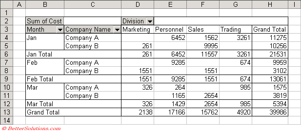Inner Field = Company Name
Outer Field = Month

The Data area will be first aggregated using the outer row field and then using each inner row field.
Inner and Outer fields work in exactly the same way.
When you have multiple fields in the same area you can change their order in the Pivot table. Select (Pivot Table > Order).

Using the Page Field

The page field can only show one item at a time.
To create a page field drag a field to the top left corner of the pivot table report.
When a Page Field has been added to your pivot table an additional button "Show Pages" will be added to your PivotTable drop-down menu.
It is possible by selecting (PivotTable > Show Pages) to display each page of the pivot table on a different worksheet.

Important

Although you can change the layout of a pivot table at any time, you cannot add or remove rows manually nor can you edit the cell values within the table.
You can quickly pivot your tables by dragging the fields to the Column and Row parts of the table.
Double clicking on any cell in the Data Area enables you to drill down to see the underlying values that have contributed to that value. This will insert a new worksheet displaying all the underlying values.
You can quickly change the layout of a pivot table once it has been displayed on a worksheet by dragging the fields to the different areas of the pivot report.
You can add more fields to the row and column sections by using the Pivot Table Field Pane.