Cell References

Instead of hard typing all the values used in your spreadsheet it is possible to use cell references as well.
This means that your spreadsheet becomes more dynamic and will change accordingly when the values in the cells change.
Any formulas that contain cell references that are entered in lowercase or mixed case (i.e. B3:H6) will be automatically changed to uppercase.
An individual cell can be referenced by an unlimited number of formulas.
A cell reference does not have to contain an operator unless you want to use it to perform an operation.

Cell references on the same worksheet

It is possible to use references to other cells that are on the same worksheet.
You can insert a cell reference into a formula by either typing the address directly or by selecting the cell with the mouse.
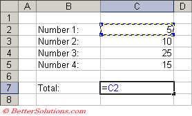
When you use the mouse to enter a cell reference the address will appear automatically and a dotted line will appear around the cell.
Once the cell (or range of cells) has been selected click back into the formula bar to enter the rest of the formula.
You can use either the formula bar to add and edit your formulas or you can edit them directly in the cell.
Select cell B2, Enter an equal sign. You can then immediately select cell D2.

The cell addresses of any cells that you select will automatically be included in your formula.
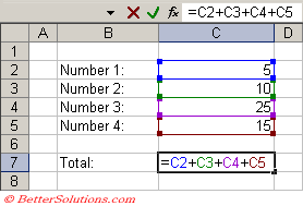
You can easily include more cell references by inserting an operator and then selecting on another cell.

Excel uses colour coding to help you manage your cell references. Each cell reference and the cell it refers to are displayed in the same colour.
The colour coding makes it very easy to identify which references in the formula match which cells on the worksheet.
If you are using the mouse to select cell references to construct your formula, only press the Enter key to confirm the final formula and not the individual cell references.

Cell references to a different worksheet in the same workbook

It is possible to use references to other worksheets in your formulas.
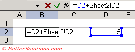
Lets assume that you have another worksheet in your workbook, called Sheet2 and that this worksheet contains a number in cell D2.
Type your formula as usual and at the point where you want to include the cell reference select that worksheet using the tabs at the bottom.
You will notice that the corresponding prefix "Sheet2!" will be automatically inserted into your formula.
Select cell D2. Do not use the mouse to click back to the original worksheet.
Before you can select the original worksheet you must either insert another operator or you must press the Enter key to confirm the formula.

If you do not enter another operator before switching back the reference will switch back to the original worksheet.
When your worksheet name contains spaces the reference must be placed within single quotes.

Cell references to a worksheet in a different workbook

It is possible to use references to cells in other workbooks. These workbooks can either be open or closed.
When the referenced workbook is open the formula is displayed as below.
The name of the workbook must be surrounded by square brackets.
If the name of the worksheet contains any spaces then the worksheet name must be enclosed in single quotes.

Notice that all cell references that refer to other workbooks are inserted as absolute references by default (see later).

If the referenced workbook is not currently open then the full directory location of the file can be used.
In this case the directory location and the workbook and worksheet name must be enclosed in single quotes.

It is possible to type in the cell references directly into your formulas although it is much easier to use the mouse.
To create a cell reference to another workbook, open the other workbook first and then use the Window drop-down menu to switch to the other workbook and select the required cell.
When you create a cell reference to a different workbook the actual data is stored in the other workbook and a copy of the data is just displayed.
The cell references will still update even when the other workbook is closed.
Every time a workbook is opened that contains cell references (or links) to other workbooks you will be prompted as to whether you want to update these links.

3D Cell References

You can use references to perform calculations on cells that span a range of worksheets in a workbook.
This technique is extremely useful if you want to summarise a group of worksheets that all have an identical layout.
=SUM(Sheet1:Sheet4!A2)
Only certain worksheet functions can be used in 3 dimensional formulas. Please refer to the 3D Formulas page for more details.

Named Ranges

It is possible to include named ranges in your formulas and using them in your formulas can often make your formulas a lot easier to understand.
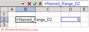
Instead of referring to a cell "=D2" (or a range of cells) using the cell address, you can actually use a descriptive name.
In the example below a worksheet named range has been created for cell "D2" called "Named_Range_D2".
You can insert named ranges into your formula by selecting (Insert > Name > Paste).

For more information on named ranges, please refer to the Named Ranges section.

Important

A quick way to copy formulas is to replace the "=" with a "#" copy and paste the formula and then replace it back.
Excel automatically adjusts formulas so when you insert a new row(s) or column(s) the formulas are adjusted to include the new row(s) or column(s). Please refer to the Automatic Formula Expansion page for more details.
You can use the formula bar to copy a formula and then to paste the formula directly into another cell. Remembering to press Escape after you have copied the formula.
If you have a lot of complicated formulas within a workbook you should try and build-in as many cross-checks as possible so the data can help to check itself.
If you have linked any of your workbooks re-naming them afterwards will create problems. You should avoid renaming any files that are referenced by other workbooks.