Formula Auditing

Also see the Functions > Troubleshooting page.

Auditing

This is the name giving to examining your formulas and making sure they are generating the correct results.
Formulas can be very complicated, especially if you combine them with named ranges, absolute and relative references as well as links to other worksheets and workbooks.
Double click on the arrows to move between the linked cells.
When you press F2 the precedents of the active cell are highlighted in Blue if the following Options(Edit tab, "Edit directly in cell) is not checked.
Understanding and stepping through complex formulas can be a real headache but there are lots of features that you can use to make this easier.
There is also a feature that lets you identify the cells responsible for any errors returned by your formulas.
They can be accessed from the (Formulas Tab).

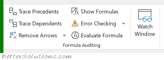Trace Precedents - Displays arrows that indicate what cells affect the value of the currently selected cell.
Trace Dependents - Displays arrows that indicate what cells are affected by the value in the currently selected cell.
Remove Arrows - Button with Drop-Down. The button removes all the arrows drawn by the trace precedents and trace dependents. The drop-down contains the commands: Remove Arrows, Remove Precedent Arrows and Remove Dependent Arrows.
Show Formulas - (Ctrl + '). Toggles the display of the formulas rather than the result.
Error Checking - Button with Drop-Down. The button displays the "Error Checking" dialog box. The drop-down contains the commands: Error Checking, Trace Error and Circular References (Auditing Toolbar). The Circular References extension will only be enabled when the active workbook contains at least one circular reference.
Evaluate Formula - Displays the "Evaluate Formula" dialog box. This allows you to step through a formula calculation. (Auditing Toolbar).
Watch Window - Displays the Watch Window.

What are the Advantages ?

Fewer Cells
Recalculation is a lot faster
Size of the workbook is reduced

What are the Disadvantages ?

Significantly harder (if not impossible) to understand and modify.

Auditing Complicated Worksheets

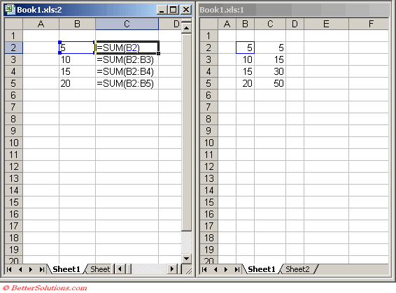
There may be times when you need to modify (or check) the formulas used in a workbook (or worksheet).
This job can be quite tedious at the best of times but to make it a bit easier it is possible to display both the formulas and the results at the same time.
To achieve this you need to open a separate window on the same workbook.
Start by opening up the workbook that contains your formulas.

Select (Window > New Window).
Select (Window > Arrange) and select Vertical.
In the left hand window press (Ctrl + ' ) or alternatively select (Tools > Options)(View tab, "Formulas").

One or More Invalid References

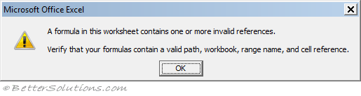
Every time I save my workbook, the following warning message keeps appearing
A formula in this worksheet contains one or more invalid references. Verify that your formulas contain a valid path, workbook, range name, and cell reference

The most common cause is an invalid reference inside a chart.

To recreate:
Create a new blank workbook
Select cells "A1:B6" on worksheet "Sheet1"
Enter the formula "=rand()" and press (Ctr + Enter)
Display the Insert Tab and select Column, Clustered Column to add a chart to Sheet1
Copy the chart and paste it onto "Sheet2"
Delete Sheet1
Right click on the chart on Sheet2 and choose "Select Data"
Press Edit under Legend Entries
You will see a #REF in the series values reference

######

This is displayed when a column is not wide enough to display the result. This is not technically an error.
Using a negative date or time.
A ##### error value occurs when the cell contains a number, date, or time that is wider than the cell or when the cell contains a date or time formula that produces a negative result. Try increasing the width of the column.
A number which is not a valid date serial number but has a date number format.

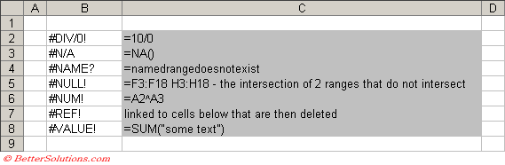
Generating Errors

It can sometimes be useful to generate different types of errors when testing your workbooks and formulas.
The following table shows you examples of formulas that will generate the necessary error values.

Finding Errors

Sometimes when you enter a formula an error will occur. This is to indicate that the formula syntax is incorrect.
If this error occurs press OK to be taken back to the formula bar. You can either correct the formula or press ESC to remove the formula completely.
This error may be caused by missing parentheses or incorrect arguments being passed to functions (e.g. passing a string when it is expecting a number).
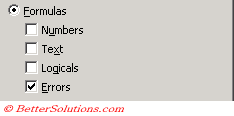
To quickly locate any cells that contain errors, select (Home tab, Find & Select > GoTo Special) and tick the Formulas, Errors checkbox.

Preventing Errors

A common method used to try and eliminate errors from appears on your worksheet is to use the ISERROR worksheet function as a wrapper.

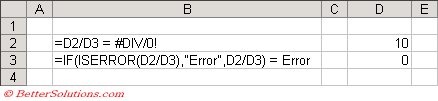The formula in cell B2 tries to divide D2 by D3, which generates an error as division by zero is not possible.
The formula in cell B3 includes the ISERROR function as a wrapper around the formula.

Debugging

If you are checking that formulas are correct, you can create a new window of the same workbook and view the values in one window and the formulas in another window. You can quickly toggle between the values and formulas by pressing ??
If you have a large number of intermediate formulas you can combine them into one large formula. The advantage of this is that recalculation of the spreadsheet is faster.
The quickest way to convert formulas to values is to move the formulas one cell to the right, and then hold down the right mouse button, when you drag them back to the original position. Choose "copy as values" from the shortcut menu ??
If you enter a large formula and it is not correct, press the OK to edit the formula, press HOME to take you to the start of the formula and enter an apostrophe. This will enter your formula as text and allow you to edit it easily

You can examine the components of a large formula by dragging the pointer to highlight part of the formula and pressing the F9 key to evaluate only the highlighted part. Remember to press the ESC key afterwards.
You can quickly select all the cells that contain formulas by choosing (Edit > GoTo > Special) and select formulas ??
The N() worksheet function is a way to include a text description into a cell containing a formula, without it affecting the formula.
You probably won't use the R1C1 notation as your default although it is very useful for checking your copied formulas. Every cell should have the same R1C1 formula.
You can retrieve data from a file without actually opening it (e.g. use the formula "=[File_Name.xls]Sheet1!A1").
You can easily display leading zeros by using a custom number format "000000". This will mean that 6 numbers are entered and any that are not entered will be zero.
You may find it helpful when editing cell references that link to other worksheets to temporarily change the worksheet name to a shorter one. Making changes with a shorter worksheet name is easier and the name can then be changed back afterwards.

Large Formulas

Quite often a formula requires a number of intermediate formulas in order to produce the correct result.
After you have got all your formulas working it is possible to eliminate the intermediate formulas and create one big "mega formula".
Formulas can only contain a maximum of 1024 characters.
If your "Mega formula" is longer than this then you should consider creating a user defined function.

Important

To prevent the misspelling of named ranges select the Name Box to insert them into your formulas.
The AutoCorrect feature will often eliminate some of the more common formula entry errors.