Variance

Variance is a measure of how spread out a set of data is in relation to the mean.
The variance is the average of the squared deviations from the mean and is always a positive number.
Lets suppose that we have two companies both with an average return of 10% a year for the past 10 years
Lets suppose that company 1 has all its yearly returns between the values of 5% and 15%
Lets suppose that company 2 has all its yearly returns dispersed over a much wider range, for example -20% and 30%
What is the likelihood of both of these companies returning 10% over the next year ?
This is very unlikely because the dispersion around the mean is an important measure.
Variance is a measure of exactly this.

Statistics > Statistical Tests > F Test page.
There are infact a whole group of statistical tests that come under the umbrella of Analysis of Variance (ANOVA)

Understanding Variance

Unfortunately you cannot just take the average distance of every point to the mean because the values above the mean will cancel out the values below the mean
For example lets suppose we have three values -5, 5 and 15
The difference between the mean is (-5-5), (5-5) and (15-5) = -10, 0, 10
The average of these values is 0 which is obviously not very useful.
One possible solution/alternative would be to square the difference before averaging the values. This would work as the square of any number is always positive.
The variance is the average of the squared deviations from the mean and is always a positive number.
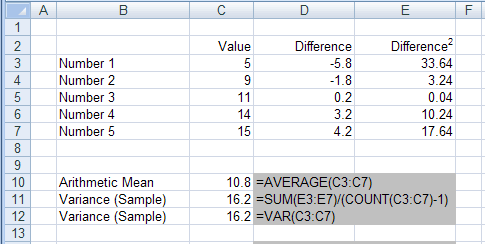
This can be quickly calculated using an Excel function.
SS

How to Calculate the Variance ?

The variance is calculated by summming the squared deviations and involves the following steps:
1) Calculate the mean of a set of values
2) Calculate the difference from the mean for each value
3) Square each difference
4) Sum up all the squares
5) Divide by the number of items in the sample, minus 1
SS - equation with T

T or (T -1)

You might come across the variance formula with the following equation

SS - equation with T-1

This formula divides the squared deviations by (T-1) instead of T
This has little impact when there a large number of observations (which there usually are)
However when the number of observations is small using (T-1) can make a big difference.
When the number of observations is small it is common to use (T-1).
In Finance you are usually working with a large number of observations so we will be using T throughout instead of (T-1).

What does the Variance tell us ?

The smaller the variance the smaller the dispersion.
The larger the variance the more spread out the observations.

Calculating the Variance on a Sample

There are three steps in finding the Variance of a distribution.
1) For each value calculate the deviation from the mean.
This is how far away each value is from the mean and can be easily obtained by subtracting each value from the mean.
2) These differences (or deviations) and then squared to ensure that they are all positive numbers.
3) The average of these (positive numbers) is the variance.
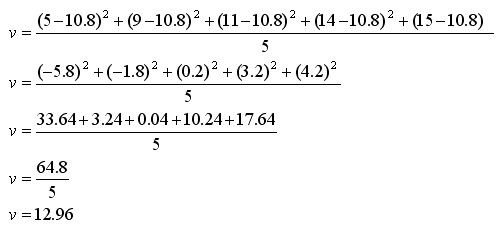
The equation for calculating the Variance is:

Uses the number minus 1

For more examples of this function please refer to the following pages:
VAR.S - (2010 - VAR) The variance based on a sample.
VARA - The variance based on a sample (including text and logical values).

Calculating the Variance on a Population

For more examples of this function please refer to the following pages:
VAR.P - (2010 - VARP) The variance based on an entire population.
VARPA - The variance based on an entire population (including text and logical values).

What is Variance Reduction ?

This is a technique that can be used to save on the number of samples required to generate an estimate to within a given error.
This refers to the ability to increase the precision of the estimates that can be obtained for a given number of iterations.
Every random variable from a simulation is associated with a variance which limits the precision of the simulation results.
To obtain a greater precision and smaller confidence intervals for the output random variable of interest, variance reduction techniques can be used.

Examples

1) Common random numbers (or correlated sampling, matched streams, matched pairs)
2) Antithetic variates
3) Control variates
4) Importance Sampling
5) Stratified Sampling

There are several different approaches that can be used.

Antithetic Variates

Two parallel simulations, one for a positive and one for a negative normal deviates producing two distributions for the underlying asset.
The arithmetic mean of the means of the two distributions is then calculated.
The large value should counter balance with the small value making the average value closer to the true value than if they were independent.
In a given sample the mean over the antithetic pairs always equals the population mean of zero. But the mean over a finite number of independent samples is almost certainly not zero.

Control Variates

This replaces the evaluation of an unknown expectation with the evaluation of the difference between the unknown Quantity and another expectation whose value is known.
The standard error from a monte carlo simulation is estimated by comparing the unknown value to be calculated against a value that is sampled but analytically known.

Importance Sampling

Also called bias sampling
This tries to generate more samples from the area that is most important.
For a random process variables are usually defined in probability distribution functions.
The calculas associated with probability distribution functions can be difficult to solve analytically.
So the monte carlo approximations turn calculus integration into algebraic summation.

Stratified Sampling

The probability distribution is divided into ranges with a sample being taken from each range according to its probability.
Ensures that fixed proportions of the samples fall within specified ranges

Martingale Variance Reduction

This involves simulteneous generation of martingales with the simulated price path
Martingales are random paths with a zero expectation (MVR variants)
The MVRs are combined linarly and then subtracted from the simulated price
As the variants average to zero, they will not affect the estimated value from monte carlo simultation
If the linear combination is chosen carefully then the standard error will be reduced.

Low Discrepancy Sequences

Discrepancy measures the uniformity of a sequence of points
low discrepancy signifies equally spaced points
This makes use of equally spaced points instead of random points which often wastes time due to clustering