VBA Code

Find the Last Populated Cell

ActiveSheet.UsedRange.Rows.Count 
ActiveSheet.UsedRange.Columns.Count 
Range("A1048576").End(xlUp).Row 

Another way is to use VBA to reset the CutCopyMode property. This doesn't work if macros are disabled.

Sub Workbook_SheetSelectionChange(ByVal sh As Object, _ 
                                  ByVal Target As Range) 
   Application.CutCopyMode = False 
End Sub 

What is the difference between UsedRange and CurrentRegion

UsedRange - the cell range of all the used cells on the worksheet.
CurrentRegion - the cell range inside blank rows and columns.

ActiveSheet.UsedRange.Row 
ActiveSheet.ActiveCell.CurrentRegion.Select 

What is the difference between Range.Value and Range.Value2

The Value2 Property does not recognise (and convert into) the VBA Currency data type or the VBA Date data type.
Range.Value - This returns the formatted value.
Range.Value2 - This returns the actual numerical value without formatting.

Empty Cells

The best way to test if a cell is empty is to use the IsEmpty() function.

If VBA.IsEmpty = False Then 

Testing for a zero-length string will be true when a formula returns a zero-length string

If rgeCell.Value <> "" Then 

No Cell Object

There is no Cell object nor is there a Cells collection.
Individual cells are treated as Range objects that refer to one cell.

Contents of a Cell

The easiest way to find what the contents of a cell are is to use the Visual Basic TypeName function

Range("A1").Value = 100 
Range("B1").Value = VBA.TypeName(Range("A1").Value)  = "Double" 

Range("A2").Value = #1/1/2006# 
Range("B2").Value = VBA.TypeName(Range("A2").Value)  = "Date" 

Range("A3").Value = "some text" 
Range("B3").Value = VBA.TypeName(Range("A3").Value)  = "String" 

Range("A4").Formula = "=A1" 
Range("B4").Value = VBA.TypeName(Range("A4").Value)  = "Double" 

Text Property

You can assign a value to a cell using its Value property.
You can give a cell a number format by using its NumberFormat property.
The Text property of a cell returns the formatted appearance of the contents of a cell.

Range("A1").Text = "$12,345.00" 

Range Object

The Range object can consist of individual cells or groups of cells.
Even an entire row or column is considered to be a range.
Although Excel can work with three dimensional formulas the Range object in VBA is limited to a range of cells on a single worksheet.
It is possible to edit a range either using a Range object directly (e.g. Range("A1").BackColor ) or by using the ActiveCell or Selection methods (e.g. ActiveCell.BackColor )

Cells Property

Application.Cells 
ActiveSheet.Cells 
ActiveCell 
Cells 

When the cells property is applied to a Range object the same object is returned.
It does have some uses though:
     ● Range.Cells.Count - The total number of cells in the range.
     ● Range.Cells(row, column) - To refer to a specific cell within a range.

ActiveSheet.Cells(2,2) = ActiveSheet.Range("B2") 

• To loop through a range of cells

For irow = 1 to 4 
   For icolumn = 1 to 4 
      ActiveSheet.Cells(irow,icolumn).Value = 10 
   Next icolumn 
Next irow 

Dim objRange As Range 
Set objRange = ActiveSheet.Range(ActiveSheet.Cells(1,4), ActiveSheet.Cells(2,6)) 

Cells automatically refer to the active worksheet.
If you want to access cells on another worksheet then the correct code is:

Range( Worksheets(n).Cells(""), Worksheets(n).Cells("") ) 

Range Property

Application.Range 
ActiveSheet.Range 
Range 

When Range is not prefixed and used in a worksheet module, then it refers to that specific worksheet and not the active worksheet.

Selection Property

Selection will return a range of cells
Be aware that the Selection will not refer to a Range object if another type of object, such as a chart or shape is currently selected.
Using the Selection object performs an operation on the currently selected cells.
If a range of cells has not been selected prior to this command, then the active cell is used.

Selection.Resize(4,4).Select 

It is always worth checking what is currently selected before using the Selection property.

If TypeName(Selection) = "Range" Then 
End If 

Relative References

It is important to remember that when a Cells property or a Range property is applied to a Range object, all the references are relative to the upper-left corner of that range.

ActiveSheet.Range("B2:D4").Cells(2,2) = ActiveSheet.Range("C3") 
ActiveSheet.Range("B2:D4").Range("B2") = ActiveSheet.Range("C3") 

ActiveCell returns a reference to the currently active cell
This will only ever return a single cell, even when a range of cells is selected.
The active cell will always be one of the corner cells of a range of cells. - will it what if you use the keyboard ??

Total number of populated cells

iTotal = Application.CountA(ActiveSheet.Cells) 

Window Object Only

This property applies only to a window object
This will enter the value 12 into the range that was selected before a non-range object was selected.

ActiveWindow.RangeSelection.Value = 12 

Window.RangeSelection property is read-only and returns a Range object that represents the selected cells on the worksheet in the active window.
If a graphic object is active or selected then this will returns the range of cells that was selected before the graphic object was selected.

Counting

Dim ltotal As Long 
ltotal = Cells.Count 'returns a long  

Dim dbtotal As Double 
dbtotal = Cells.CountLarge ' returns a double  

Range of a Range

It is possible to treat a Range as if it was the top left cell in the worksheet.
This can be used to return a reference to the upper left cell of a Range object
The following line of code would select cell "C3".

Range("B2").Range("B2").Select 

Range("B2").Cells(2).Select 

Remember that cells are numbered starting from A1 and continuing right to the end of the row before moving to the start of the next row.

Range("B2").Cells(2,2).Select 

An alternative to this is to use the Offset which is more intuitive.

Range.Address

The Address method returns the address of a range in the form of a string.

Range("A1:B3").Address = "$A$1:$B$3" 
Range("A1:B3").Address(False,False) = "A1:B3" 

Using the parameters allows you to control the transformation into a string (absolute vs relative).

Range.Address([RowAbsolute], 
              [ColumnAbsolute], 
              [ReferenceStyle], 
              [External], 
              [RelativeTo]) As String 

RowAbsolute - True or False, default is True
ColumnAbsolute - True or False, default is True
ReferenceStyle - xlReferenceStyle.xlA1
External - True to return an external reference, default is false
RelativeTo - Range representing a relative to cell. Only relevant when ReferenceStyle = xlR1C1

Range.AddressLocal

This is similar to Address but it returns the address in the regional format of the language of the particular country.

Cells.Replace SearchFormat:=True, ReplaceFormat:=True 
lLastRowNo = ActiveCell.End(xlDown).Row 

Moving large amounts of data quickly

Dim vArray As Variant 

vArray = Range("A1").Resize(10,10) 
Range("H6").Resize(10,10) = vArray 

Obtaining the cell reference of the active cell

Dim lrownumber As Long 
Dim icolumnno As Integer 

lrownumber = ActiveCell.Row 
icolumnno = ActiveCell.Column 
Call MsgBox("The currently active cell is " & lrowno & " , " & icolumnno) 

Makes the active cell the top left cell in the window

ActiveCell.Select 
ActiveWindow.ScrollColumn = ActiveCell.Column 
ActiveWindow.ScrollRow = ActiveCell.Row 

Selection

Selection.PasteSpecial Paste:=xlValues 
Selection.Copy 
Selection.Cut 
Set objRange = Selection 
Selection.Rows.Count 

Looping through all the selected cells

For Each objCell In Selection.Cells 

Next objCell 

Range of cells currently selected

ifirstcol = Range(Selection.Address).Column 
inoofcols = Range(Selection.Address).Column + Selection.Columns.Count 
lfirstrow = Range(Selection.Address).Row 
lnoofrows = Range(Selection.Address).Row + Selection.Rows.Count 
Selection.Font.Size = 12 
If TypeName(Selection) = "Range" Then MsgBox("More than one cell currently selected") 

Formatting

Call MsgBox( Range("A3").Font.ColorIndex ) 
Call MsgBox( Range("A3").Interior.ColorIndex ) 
If (Range("A3").Font.ColorIndex < 0) Then Call MsgBox (" When ?") 
If (Range("A3").Interior.ColorIndex < 0) Then Call MsgBox (" When ?") 
Range("A2").Font.Bold = True 
Range("A4:D10").NumberFormat = "mmm-dd-yyyy" 

Looping Through Cells

Dim rgeCell As Cell 

For Each rgeCell In Range("A1:D30").Cells 
   rgeCell.Value = 20 
Next rgeCell 
Dim rgeCurrent As Range 

Do While Not IsEmpty(rgeCurrent) 
   'do something
   Set rgeCurrent = rgeCurrent.Offset(1,0) 
Loop 

You can prevent the user scrolling around a worksheet by defining the scroll area. Worksheets("Sheet1").ScrollArea = "A1:D400". To set the scrolling back to normal just assign the ScrollArea to an empty string. Note that this setting is not saved so it may be necessary to include it in the WorkBook_Open() event procedure.
You can quickly assign an Excel Range of cells to an array and visa-versa. Be aware that these arrays will start at 1 and not 0. vArrayName = Range(---).Value.

Determining a Cell Datatype

Help determine the type of data contained in a cell.
This accepts a range of any size but only operates on the upper left cell in the range.

Function CellType(Rng) 
'   Returns the cell type of the upper left
'   cell in a range
    Application.Volatile 
    Set Rng = Rng.Range("A1") 
    Select Case True 
        Case IsEmpty(Rng): CellType = "Blank" 
        Case Application.IsText(Rng): CellType = "Text" 
        Case Application.IsLogical(Rng): CellType = "Logical" 
        Case Application.IsErr(Rng): CellType = "Error" 
        Case IsDate(Rng): CellType = "Date" 
        Case InStr(1, Rng.Text, ":") <> 0: CellType = "Time" 
        Case IsNumeric(Rng): CellType = "Value" 
    End Select 
End Function 

Save Shape As PNG

Sub SaveShapeAsPicture() 
Dim cht As ChartObject 
Dim ActiveShape As Shape 
Dim UserSelection As Variant 

  On Error GoTo ErrorHandler 
    Set UserSelection = ActiveWindow.Selection 
    Set ActiveShape = ActiveSheet.Shapes(UserSelection.Name) 

'Create a temporary chart object (same size as shape)
  Set cht = ActiveSheet.ChartObjects.Add( _ 
    Left:=ActiveCell.Left, _ 
    Width:=ActiveShape.Width, _ 
    Top:=ActiveCell.Top, _ 
    Height:=ActiveShape.Height) 

'Format temporary chart to have a transparent background
  cht.ShapeRange.Fill.Visible = msoFalse 
  cht.ShapeRange.Line.Visible = msoFalse 
    
'Copy/Paste Shape inside temporary chart
  ActiveShape.Copy 
  cht.Activate 
  ActiveChart.Paste 
   
'Save chart to User's Desktop as PNG File
  cht.Chart.Export Environ("USERPROFILE") & "\Desktop\" & ActiveShape.Name & ".png" 

'Delete temporary Chart
  cht.Delete 

'Re-Select Shape (appears like nothing happened!)
  ActiveShape.Select 

Exit Sub 
ErrorHandler: 
End Sub 

Save Range as JPG

Sub SaveRangeAsPicture() 
Dim cht As ChartObject 
Dim ActiveShape As Shape 

  On Error GoTo ErrorHandler 
'Confirm if a Cell Range is currently selected
  If TypeName(Selection) <> "Range" Then 
    MsgBox "You do not have a single shape selected!" 
    Exit Sub 
  End If 

'Copy/Paste Cell Range as a Picture
  Selection.Copy 
  ActiveSheet.Pictures.Paste(link:=False).Select 
  Set ActiveShape = ActiveSheet.Shapes(ActiveWindow.Selection.Name) 
  
'Create a temporary chart object (same size as shape)
  Set cht = ActiveSheet.ChartObjects.Add( _ 
    Left:=ActiveCell.Left, _ 
    Width:=ActiveShape.Width, _ 
    Top:=ActiveCell.Top, _ 
    Height:=ActiveShape.Height) 

'Format temporary chart to have a transparent background
  cht.ShapeRange.Fill.Visible = msoFalse 
  cht.ShapeRange.Line.Visible = msoFalse 
    
'Copy/Paste Shape inside temporary chart
  ActiveShape.Copy 
  cht.Activate 
  ActiveChart.Paste 
   
'Save chart to User's Desktop as PNG File
  cht.Chart.Export Environ("USERPROFILE") & "\Desktop\" & ActiveShape.Name & ".jpg" 

'Delete temporary Chart
  cht.Delete 
  ActiveShape.Delete 

'Re-Select Shape (appears like nothing happened!)
  ActiveShape.Select 

Exit Sub 
ErrorHandler: 
End Sub 

Activate vs Select

There is a difference between activating a range and selecting a range.
The following means that the cells "A1:D4" are selected and since "B2" is contained in the cell range "A1:D4" it is the active cell within a larger selection.

Range("A1:D4").Select 
Range("B2").Activate 

The following means that the cells "A1:D4" are selected but since "D6" is not contained in cell range "A1:D4", the cell "D6" is then selected.

Range("A1:D4").Select 
Range("D6").Activate 

Both methods can only be used to select cells on the active worksheet.

Range to Array

The quickest way to populate an array with values in a cell range is to use a simple Variant data type.
You do not need to define the size of the array before it is populated.
This is only possible when the variable is defined as a Variant.

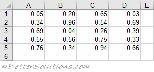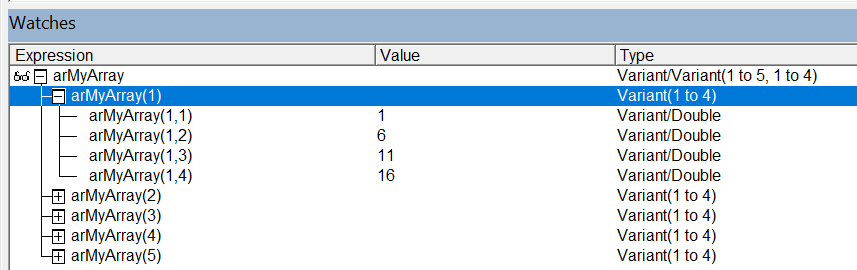
The array will always be 2 dimensional, it starts at 1 (not 0) and is always rows then columns.

Rows and Columns:

Dim arMyArray As Variant 
arMyArray = Range("A1:D5").Value 

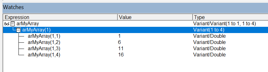
One Row:

Dim arMyArray As Variant 
arMyArray = Range("A1:D1").Value 

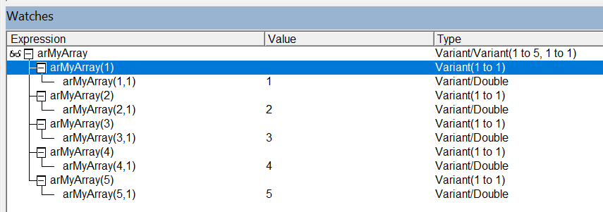
One Column:

Dim arMyArray As Variant 
arMyArray = Range("A1:A5").Value 

Array to Range

The quickest way to populate a range with the contents of an array is to define the Value equal to the array.

Rows and Columns:
If you have a 2 dimensional array that you want to display on a worksheet you can assign the array to a Range.Value.
If the array has been populated with (rows, columns) the array can be assigned as it is.

Dim arValues As Variant 
ReDim arValues(1 To 2, 1 To 3) 
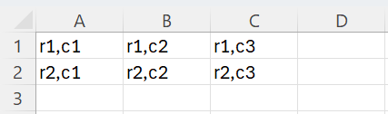
arValues(1, 1) = "r1,c1" 
arValues(1, 2) = "r1,c2" 
arValues(1, 3) = "r1,c3" 

arValues(2, 1) = "r2,c1" 
arValues(2, 2) = "r2,c2" 
arValues(2, 3) = "r2,c3" 

Range("A1:C2").Value = arValues 

This will create the following table.

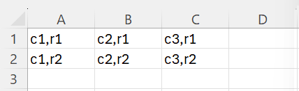
If the array has been populated with (columns, rows) the array needs to be transposed first.

Dim arValues As Variant 
ReDim arValues(1 To 3, 1 To 2) 
arValues(1, 1) = "c1,r1" 
arValues(1, 2) = "c1,r2" 

arValues(2, 1) = "c2,r1" 
arValues(2, 2) = "c2,r2" 

arValues(3, 1) = "c3,r1" 
arValues(3, 2) = "c3,r2" 

arValues = Application.WorksheetFunction.Transpose(arValues) 
Range("A1:C2").Value = arValues 

This will create the following table.

One Row:
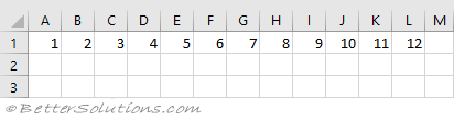
Note that this will create a horizontal array that will populate a row across the worksheet.

Dim arValues As Variant 
arValues = VBA.Array(1, 2, 3, 4, 5, 6, 7, 8, 9, 10, 11, 12) 
Range("A1:L1").Value = arValues 

This will create a table across the worksheet.

One Column:
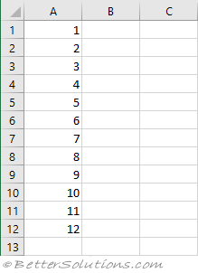
If you want to create a vertical array that will populate a column down the worksheet then you must transpose the array before assigning it to the Range.

Dim arValues As Variant 
arValues = VBA.Array(1, 2, 3, 4, 5, 6, 7, 8, 9, 10, 11, 12) 
arValues = Application.WorksheetFunction.Transpose(arTesting) 
Range("A1:A12").Value = arValues 

This will create a table down the worksheet.

Empty Value

Dim aMyArray As Variant 
aMyArray = Range("A1").Value 

aMyArray has a value Empty if cell "A1" is empty

aMyArray = Range("A1").Value 

aMyArray has the value if cell "A1" contains a value

Row and Column Vectors

Dim aMyArray As Variant 
aMyArray = Range("A1:B1")    'row vector  
aMyArray(1,1) = 1 
aMyArray(1,2) = 2 

Dim aMyArray As Variant 
aMyArray = Range("A1:A2")    'column vector  
aMyArray(1,1) = 1 
aMyArray(2,1) = 2 

Transposing the Array

VBA > Arrays > Transposing

Remember

Excel reads FROM ranges a lot faster than it writes TO ranges.

Value or Value2

The Value2 property does not recognise (and convert into) the VBA Currency data type or the VBA Date data type.
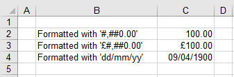
The difference between these two properties is best explained with a simple example.
Enter the number 100 into the cells "C2", "C3" and "C4" and apply the corresponding formatting.

Using Excel Number Format

Cell "C2" has been formatted using the number format "#,##0.00".
Run the following code and when you get to the Stop statement open the Watches window and the Immediate window.

Call ValueOrValue2("C2") 

Public Sub ValueOrValue2(ByVal sAddress As String) 
   Dim vCell_value As Variant 
   Dim vCell_value2 As Variant 
   vCell_value = Range(sAddress).Value 
   Debug.Print vCell_value 
   vCell_value2 = Range(sAddress).Value2 
   Debug.Print vCell_value2 
   Stop 
End Sub 

Notice that the Type for both these local variables is "Variant/Double".

Using Excel Currency Format

Cell "C3" has been formatted using the currency format "£#,##0.00".
Run the following code and when you get to the Stop statement open the Watches window and the Immediate window.

Call ValueOrValue2("C3") 

Notice that the Type for the "Value" property is "Variant/Currency".
And the Type for the "Value2" property is still "Variant/Double".
When you use the "Value2" property in conjunction with cells formatted as Currency they will be recognised as a Double and not as a Currency.
The VBA Currency data type stores numbers as a fixed point number.
If you have numbers that have more than 4 decimal places then using "Value2" will be more accurate.

Using Excel Date Format

Cell "C4" has been formatted using the date format "dd/mm/yyyy".
Run the following code and when you get to the Stop statement open the Watches window and the Immediate window.

Call ValueOrValue2("C4") 

Notice that the Type for the "Value" property is "Variant/Date". This corresponds to what is displayed in the Immediate window.
And the Type for the "Value2" property is still "Variant/Double".
When you use the "Value2" property in conjunction with cells formatted as Dates they will be recognised as a Double and not as a Date..
The VBA Date data type stores numbers as decimal.
The only time it makes sense to use .Value instead of .Value2 is if you want to detect a date in a cell using the VBA.IsDate() function.

Dim vCell As Variant 
vCell = Range("A1").Value 
'This creates a sub type of Date which can be detected by the VBA.IsDate function
If (VBA.IsDate(vCell) = True) Then 
End If 

If you use Value2 in the above example then a date will be converted to a Double data type which is not recognised by the VBA.IsDate function.
Value has an optional parameter of type xlRangeValueDataType
If you pass in Value(xlRangeValueDataType.xlRangeValueDefault) you will get back an object representing the value of the cell.
Both of these methods will return an array if the Range contains multiple cells.

Range("D3").Value2 = Range("A3").Value2 + Range("C7").Value2 

Entering data on the active worksheet

If you want to enter data onto the active worksheet then you can use any of the following.

ActiveSheet.Range("D3").Value = "some text" 
ActiveSheet.Cells(3,4).Value = 200 
Range("D3").Value = "some text" 
Range("A2").Value = Range("B4").Value + 20 
Cells(7,2).Value = 25 

This enters the number 60 into all the cells in the range "A1:B10".

Range("A1:B10").Value = 60 

This enters the number 18 into the four cells "A1", "B1", "C1" and "D1".

Range("A1,B1,C1,D1").Value = 18 

This enters the number 5 in all the cells that are the intersection of the two ranges.

Range("A1:B10 A1:D10").Value = 5 

Entering data on a different worksheet

It is good practice to always qualify the worksheet, whether it is the active worksheet or a different worksheet.

Worksheets("Sheet1").Range("A2").Value = 20 
Sheets("Sheet1").Range("B2").Value = 30 
Sheets(2).Cells(3,3).Text = "some text" 

Remember the difference between "Worksheets" and the "Sheets" collection.
The "Sheets" collection includes all sheets, including Chart sheets.

ActiveCell

The ActiveCell is always a single cell and is the cell that contains the cell pointer.
This property always refers to the active worksheet or window.
If you select several cells on a worksheet, then these cells are considered a selection. One of these cells is the active cell.
A cell does not have to be active in order for it to be edited.
Trying to obtain a reference to the ActiveCell will fail if a Chart Sheet is currently active.

Dim objCell As Range 

Set objCell = Application.ActiveCell 
Set objCell = ActiveWindow.ActiveCell 
Set objCell = ActiveCell 

If a range of cells is selected, the active cell will be in one of the corners and will depend on how the range was selected.
ActiveCell returns Nothing if no worksheet is displayed in the active window.

Selection

The Selection property will references whatever is currently selected in the active workbook.
This could be a Range, Shape, Chart, anything

Application.Selection 
Selection 

RangeSelection

This refers to the selected cells on the worksheet in the specified window, even when a graphic object is selected.
This property applies to a Window object.

ActiveWindow.RangeSelection 

This can be useful when you want to refer to the range that was selected before a non-range object was selected.

Using the Cells collection

A common way to refer to particular cells on a worksheet is to use the Cells property.
This enters the number 10 into cell "B2" on the active worksheet.

ActiveSheet.Cells(rowindex, columnindex).value = 10 
ActiveSheet.Cells(2, 2).Value = 10 

You can also use the Cells property to refer to a particular cell on a worksheet or in a range
Cells are numbered starting at the left and continuing to the right and then down to the next row.

ActiveSheet.Cells(500).Value = 10 

Removing Data

Using the ClearContents method, removes just the value from a cell and not the cell formatting.

Sheets("Sheet1").Cells.ClearContents 
Range("C1:E6").ClearContents 

Sorting Data

more info

Selecting Individual Cells

Cannot select a cell unless that particular worksheet is displayed/active
If using the notation Range("An") is not convenient you can use Cells(rows,columns) instead.
The row and column indexes both start at 1 for Cells(row, column)
It is also possible to use the GoTo dialog box.

Range("B1").Select 

Cells(RowIndex, ColumnIndex).Select 
Cells(1, 2).Select 
Cells(1, "B").Select   'not guaranteed ???  

Application.GoTo

This is comparable to the select method except the range is passed as a parameter
If the range is on another worksheet then that worksheet will be automatically selected.
GoTo is a method that causes Excel to select a range of cells and activate the corresponding workbook.
It takes an optional Object parameter (either String or Range).
It also takes an optional second Object parameter that can be set to True to indicate if you want Excel to scroll the window so that the selection is in the top-left corner.

Application.GoTo Range("B3") 
Application.GoTo Reference:=Range("A2") 
Application.GoTo ("R3C2") 
Application.GoTo ("Sheet1!R3C2") 
Application.GoTo (Range("A2"),True) 
Application.GoTo (Range("A2","B3"),True) 

This is also has an optional scrolling parameter ??
The following line of code is not allowed.

Range(Cells(2,3)).Select 

Selecting a Range (or Multiple Cells)

Range("A1:D4").Select 
Range("A1", "D4").Select 'This is exactly the same as the above line  
Range("A1,D4").Select 'This selects just the 2 cells  

Range("A1", "G3").Select 
Range("B1:C10").Select 
Range("A1:B2, C3:D4").Select 
Range("A1:B4", "D3:G6").Select 
Range( Cells(2,3), Cells(5,6) ).Select 
Worksheets("Sheet3").Range("A1:B10, C2:D40").Select 
Application.Intersect(Range("A2"), Range("D10")) 
Range("C1:C10 A6:E6").Select 
Application.Union(Range("A1:G10"), Range("B6:D15")) 

You can also use the following abbreviation although it is not recommended:

Range("A1:B3").Select 
[A1:B3].Select 

Selecting the whole worksheet

ActiveSheet.Cells.Select 

Selecting a Different worksheet

The following line of code will not work unless Sheet1 is currently selected.

Worksheets("Sheet1").Range("A2").Select 

You must select the worksheet first and then select the range.

Selecting using the Current Selection

Using the Selection object performs an operation on the currently selected cells.
If a range of cells has not been selected prior to this command, then the active cell is used.

Selection 

Selecting using the Active Cell

The ActiveCell is often used and refers to the cell that is currently selected.
You can also easily obtain the cell address of the active cell.

ActiveCell.End(xlDirection.xlDown).Select 
Call MsgBox( ActiveCell.Column & ActiveCell.Row ) 

Selecting the CurrentRegion or UsedRange

The CurrentRegion property setting consists of a rectangular block of cells surrounded by one or more blank rows or columns.
The UsedRange is the range of all non-empty cells.

ActiveSheet.ActiveCell.CurrentRegion.Select 
ActiveSheet.UsedRange.Select 

Selecting using Relative References

You can use the Range property of a Range object to create a relative reference to the Range object (e.g. Range("C3").Range("B2") = D4).
If you are using Range("A4".Cells(2,2)) to obtain a relative reference it is marginally faster to use Range("A4")(2,2).

Range("A2").End(xlDirection.xlDown).Select 
Range("A1:D10").Cells(6).Select 

Selecting Rows and Columns

Range("C:C").Select 
Range("7:7").Select 
Range("2:2,4:4,6:6").Select 
Range("A;A,C;C,E;E").Select 

Range.SpecialCells Method

This method returns a range that represents all the cells that match a particular criteria

Range.SpecialCells(Type, Value) 

Type - The type of cells to select from the xlCellType enumeration.
Value - This is an additional argument that is required when Type is xlCellTypeConstants or xlCellTypeFormulas.
The default is to select all constants and formulas.

objBlankCells = Selection.SpecialCells(Type:=xlCellType.xlCellTypeBlanks) 

The following line selects the last "used" cell on the worksheet

ActiveSheet.Cells.SpecialCells(Type:=xlCellType.xlCellTypeLastCell) 

xlCellTypeConstants or xlCellTypeFormulas.

Using this method will generate an error if there are no cells currently selected.
The following line creates a subset range containing all the cells that contain formulas.

objFormulaCells = Selection.SpecialCells(Type:=xlCellType.xlCellTypeFormulas, _ 
                                         Value:=xlSpecialCellsValue.xlNumbers) 

The following line creates a subset range containing all the cells that contain constants

objConstantCells = Selection.SpecialCells(Type:=xlCellType.xlCellTypeConstants, _ 
                                          Value:=xlSpecialCellsValue.xlNumbers) 

The following line clears all constants from a worksheet

objWorksheet.Cells.SpecialCells(Type:=xlCellType.xlCellTypeConstants, _ 
                                Value:=xlSpecialCellsValue.xlNumbers).ClearContents 

Selecting all non blank cells on a sheet

Public Sub AllNonBlank() 
   Application.Union(ActiveSheet.Cells.SpecialCells(Type:=xlCellType.xlCellTypeFormulas, 
                                                    Value:=xlSpecialCellsValue.xlErrors + _ 
                                                           xlSpecialCellsValue.xlLogical + _ 
                                                           xlSpecialCellsValue.xlNumbers + _ 
                                                           xlSpecialCellsValue.xlTextValues), _ 
                     ActiveSheet.Cells.SpecialCells(Type:=xlCellType.xlCellTypeConstants, _ 
                                                    Value:=23)).Select 
End Sub 

Selecting all cells in a range that contain an error

This will select any cells that contain: #CALC!, #DIV/0, #FIELD!, #N/A, #NAME?, #NULL!, #NUM!, #REF!, #SPILL!, #VALUE!.

Public Sub CellsWithErrors 
   Range("A1:A16385").SpecialCells(xlCellType.xlCellTypeFormulas, xlSpecialCellsValue.xlErrors).Select 
End Sub 

KeyStroke Equivalents

The macro recorder does not record any keystrokes you use to select a range of cells.
This line of code is equivalent to pressing (Ctrl + Shift + 8).

ActiveCell.CurrentRegion.Select 

Multiple Selected Ranges

A Range object can comprise of multiple separate ranges.
Most properties and methods that refer to a range object take into account only the first rectangular area of the range.
You can use the Areas property to determine if a range contains multiple areas

If (Selection.Areas.Count > 1) Then 
End If 

Excel will actually allow multiple selections to be identical.
You can hold down the Ctrl and click cell "A1" five time.
The selection will have five identical areas.

Protecting Cells

This just prevents the cells from being edited

Dim objRange As Excel.Range 

If (objRange.Locked = True) Then 
   'all cells in range are locked
End If 

If (objRange.Locked = False) Then 
   'all cells in range are not locked
End If 

If (objRange.Locked = null) Then 
   'cells in range have a combination of locked and unlocked
End If 

GoTo Dialog

If Type is either xlCellTypeConstants or xlCellTypeFormulas, this argument is used to determine which types of cells to include in the result.
These values can be added together to return more than one type.
The default is to select all constants or formulas, no matter what the type.

Comments

ActiveSheet.Cells.SpecialCells(Type:=xlCellType.xlCellTypeComments).Select 
Selection.SpecialCells(xlCellType.xlCellTypeComments).Select 

Constants

Selection.SpecialCells(xlCellType.xlCellType.Constants, 23).Select 
ActiveSheet.Cells.SpecialCells(Type:=xlCellType.xlCellTypeConstants, _ 
                               Value:=xlSpecialCellsValue.xlNumber).Select 

Formulas

Selection.SpecialCells(xlCellType.xlCellTypeFormulas,3).Select 
ActiveSheet.Cells.SpecialCells(Type:=xlCellType.xlCellTypeFormulas, _ 
                               Value:=xlSpecialCellsValue.xlNumber).Select 

Blanks

Selection.SpecialCells(xlCellType.xlCellTypeBlanks).Select 

CurrentRegion

Selection.CurrentRegion.Select 

CurrentArray

Selection.CurrentArray.Select 

Objects

ActiveSheet.DrawingObjects.Select 

Row Differences

Selection.RowDfferences(ActiveCell).Select 

Column Differences

Selection.ColumnDifferences(ActiveCell).Select 

Precedents

Selection.DirectPrecedents 

Dependents

Selection.DirectDependents 

Last Cell

Selection.SpecialCells(xlCellType.xlCellTypeLastCell).Select 

Visible Cells Only

Selection.SpecialCells(xlCellType.xlCellTypeVisible).Select 

Conditional Formatting

ActiveCell.SpecialCells(xlCellType.xlCellTypeAllFormatConditions).Select 

Data Validation

ActiveCell.SpecialCells(xlCellType.xlCellTypeAllValidation).Select 

Application.Intersect

Returns a Range object that represents the rectangular intersection of two or more ranges.

This example selects the intersection of two named ranges, rg1 and rg2, on Sheet1. If the ranges don't intersect, the example displays a message.

Worksheets("Sheet1").Activate 
Set isect = Application.Intersect(Range("rg1"), Range("rg2")) 
If isect Is Nothing Then 
    MsgBox "Ranges do not intersect" 
Else 
    isect.Select 
End If 

Application.Union

Returns the union of two or more ranges.
This example fills the union of two named ranges, Range1 and Range2, with the formula =RAND().

Worksheets("Sheet1").Activate 
Set bigRange = Application.Union(Range("Range1"), Range("Range2")) 
bigRange.Formula = "=RAND()" 

Sub Testing_Selection() 
Dim lrowno As Long 
Dim icolno As Integer 
   Dim objObject As Excel.Application 
   Dim iareatotal As Integer 
   Dim iareacount As Integer 
   Dim objFinalSelection As Excel.Range 
   Dim objUnionSelection As Excel.Range 
    Dim objcellfirst As Excel.Range 
    Dim objcellstartofrow As Excel.Range 
    Dim objSelection As Excel.Range 
         
    Set objObject = Application 
    
    objObject.Range("C4:F15").Select 
    objObject.Selection.FormulaArray = "=RAND()" 

    Set objUnionSelection = objObject.Range("E10") 
    Set objUnionSelection = Union(objUnionSelection, objObject.Range("F13")) 
    objUnionSelection.Select 
         
    Set objSelection = objObject.Selection 
    iareatotal = objSelection.Areas.Count 
         
    For iareacount = 1 To iareatotal 
         
        lrowno = objSelection.Areas(iareacount).Row 
        icolno = objSelection.Areas(iareacount).Column 
    
        Set objcellfirst = objObject.Cells(lrowno, icolno) 
        Set objcellstartofrow = objSelection.Areas(iareacount). 
            Offset(0, objObject.Cells(lrowno, icolno).CurrentRegion.Column - icolno) 
        Set objFinalSelection = objcellstartofrow.Resize( 
             objSelection.Areas(iareacount).Rows.Count, objcellfirst.CurrentRegion.Columns.Count) 
        
        If iareacount = 1 Then 
           Set objUnionSelection = objFinalSelection 
        Else 
           Set objUnionSelection = Union(objUnionSelection, objFinalSelection) 
        End If 
    
    Next iareacount 
    
    objUnionSelection.Select 
End Sub 

Inserting Cells

Range("B2:F5").Insert(xlInsertShiftDirection.xlShiftDown) 
Range("B2:F5").Insert(xlInsertShiftDirection.xlShiftToRight) 

Deleting Cells

This deletes the cells in the range "B2:F2".

Range("B2:F5").Delete(xlDeleteShiftDirection.xlShiftUp) 
Range("B2:F5").Delete(xlDeleteShiftDirection.xlShiftToLeft) 

If the Shift argument is omitted then Excel will guess the best direction based on the shape of the range.

Clearing Data

ActiveCell.CurrentRegion.ClearContents 

Selection.Delete

Even with displayalerts = false you will get the following prompt if the selection currently has a filter applied to it.
SS
Delete entire row ?

Cutting and Pasting ranges of cells

You can cut and paste a single value using either of the following lines of code:

Range("A2").Cut Destination:=Range("D2") 
Range("A2").Cut Range("D2") 

The Cut method also has an optional destination argument.
It is possible to cut and paste a range of cells:

Range("A2:B4").Select 
Selection.Cut 
Range("D7").Select 
ActiveSheet.Paste 

Alternatively you can combine this to a single line.
This is possible because the Cut method can take an optional argument that can represent the range to be cut to. The next two lines are equivalent.

Range("A2:B4").Cut Destination:=Range("D7") 
Range("A2:B4").Cut Range("D7") 

Application.Calculate

If you are manipulating a lot of cells then it is sometimes a good idea to switch the automatic calculation off temporarily

Application.Calculate = xlCalculation.xlCalculationManual 
'manipulating a lot of cells
Application.Calculate = xlCalculation.xlCalculationAutomatic 

Copying

Excel > Charts > VBA Code > Copying
Excel > Illustrations > VBA Code > Copying
Word > Paragraphs > VBA Code

Copying and Pasting a single value

The most intuitive way to copy data from one cell to another would be:

Range("A2").Select 
Selection.Copy 
Range("D2").Select 
ActiveSheet.Paste 

One of the most important aspects of VBA programming is remembering that you do not have to actually select the object you want to manipulate.
The code could therefore be changed to the following.

Range("A2").Copy 
Range("D2").Select 
ActiveSheet.Paste 

There are always several ways to accomplish the same thing in VBA.
The code could be reduced to two lines using the Paste Special method.

Range("A2").Copy 
Range("D2").PasteSpecial Paste:=xlValues 

It is actually possible to condense this action into a single line.
This is possible because the Copy method can take an optional argument that can represent the range to be copied to. The next two lines are equivalent.

Range("A2").Copy Destination:=Range("D2") 
Range("A2").Copy Range("D2") 

This copies the contents of cell "D2" and places them into the active cell.

Range("D2").Copy Destination:=ActiveCell    

Copying Data between Worksheets

It is possible to copy data between worksheets.
The can be done by including a reference to a particular worksheet. If no worksheet is specified then the active worksheet is used.

Worksheets("Sheet1").Range("A2").Copy Worksheets("Sheet2").Range("D2") 

Notice that you do not have to activate the necessary worksheets.
The following line of code copies the whole block of data to a worksheet Sheet2.

Range("A2").CurrentRegion.Copy Sheets("Sheet2").Range("D2") 

Copying Data between Workbooks

It is possible to copy data between worksheets.
The can be done by including a reference to a particular worksheet. If no worksheet is specified then the active worksheet is used.

Workbooks("Wbk1.xls".Worksheets("Sheet1").Range("A2").Copy Workbooks("Wbk2.xls").Worksheets("Sheet2").Range("D2") 

Long lines of code can sometimes be difficult to understand.
Another way to perform the same task is to use variables to store the necessary range objects.

Dim rgeCopyRange As Range 
Dim rgeToRange As Range 

Set rgeCopyRange = Workbooks("Wbk1.xls").Worksheets("Sheet1").Range("A2") 
Set rgeToRange = Workbooks("Wbk2.xls").Worksheets("Sheet2").Range("D2") 
rgeCopyRange.Copy rgeToRange 

Cancelling the Copy Mode

When you copy (or Cut) a range of cells a black dotted line appears around the area to help identify it.
This can be removed by switching the CutCopy property to False.

Application.CutCopyMode = xlCutCopyMode.False 

If you do not change this property back to false then the cell range that was last copied will remain flashing on the screen.

Range("A2").Copy 
Range("D2").Select 
ActiveSheet.Paste 
Application.CutCopyMode = xlCutCopyMode.False 

You do not need to reset this property if you use a single line statement to copy and paste.

Range("A2").Copy Range("D2") 

Copying Ranges as Pictures

to copy the selected worksheet range as a picture

Selection.CopyPicture Appearance:=xlPictureAppearance.xlScreen, Format:=xlCopyPictureFormat.xlPicture 

Freeze and unfreeze references when copying

Public arFormulas() As Variant 

Public Sub Freeze() 
    arFormulas = Selection.Formula 
End Sub 

Public Sub UnFreeze() 
    If (Not Not arFormulas) = 0 Then 
        Call MsgBox ("Error: No formulas were copied. Please use the Freeze routine first.") 
        Exit Sub 
    End If 

    Selection.Resize(UBound(arFormulas, 1), UBound(arFormulas, 2)).Value = arFormulas 
End Sub 

Paste Special - Range Object

Pastes a Range from the Clipboard into the specified range.

Range("A1").PasteSpecial Paste:=xlPasteType.xlPasteValues, _ 
                         Operation:=xlPasteSpecialOperation.xlPasteSpecialOperationAdd, _ 
                         SkipBlanks:=False, _ 
                         Transpose:=False 

Paste - The part of the range to be pasted.
Operation - The paste operation.
SkipBlanks - Whether to have blank cells in the range on the Clipboard not be pasted into the destination range. The default value is False.
Transpose - Whether to transpose rows and columns when the range is pasted. The default value is False.

Paste Special - Worksheet Object

Pastes the contents of the Clipboard onto the sheet, using a specified format. Use this method to paste data from other applications or to paste data in a specific format.
You must select the destination range before you use this method. This method may modify the sheet selection, depending on the contents of the Clipboard.

ActiveSheet.PasteSpecial Format:="Text", _ 
                         Link:=True | False, _ 
                         DisplayAsIcon:=True | False, _ 
                         IconFileName:="C:\Temp\icon.bmp", _ 
                         IconIndex:=1, _ 
                         IconLabel:="Text label", _ 
                         NoHTMLFormatting:=True | False 

All the parameters are optional
Format - A string that specifies the Clipboard format of the data. msoClipboardFormat ?
Link - Whether to establish a link to the source of the pasted data. If the source data isn't suitable for linking or the source application doesn't support linking, this parameter is ignored. The default value is False.
DisplayAsIcon - Whether to display the pasted as an icon. The default value is False.
IconFileName - The name of the file that contains the icon to use if DisplayAsIcon is True.
IconIndex - The index number of the icon within the icon file.
IconLabel - The text label of the icon.
NoHTMLFormatting - Whether to remove all formatting, hyperlinks, and images from HTML. False to paste HTML as is. The default value is False. NoHTMLFormatting will only matter when Format = "HTML". In all other cases, NoHTMLFormatting will be ignored.

ActiveSheet.PasteSpecial Format:="Text" 
ActiveSheet.PasteSpecial Format:="HTML" 
ActiveSheet.PasteSpecial Format:="Microsoft Word 8.0 Document Object" 

This example pastes a Word document object and displays it as an icon.

Worksheets("Sheet1").Range("F5").Select 
ActiveSheet.PasteSpecial Format:="Microsoft Word 8.0 Document Object", _ 
                         DisplayAsIcon:=False, 

Paste - Worksheet Object

Pastes the contents of the Clipboard onto the sheet.
If you don't specify the Destination argument, you must select the destination range before you use this method.
This method may modify the sheet selection, depending on the contents of the Clipboard.

Worksheets("Sheet1").Range("C1:C5").Copy 
ActiveSheet.Paste Destination:=Worksheets("Sheet1").Range("A2"), _ 
                  Link:=False 

Destination - A Range object that specifies where the Clipboard contents should be pasted. If this argument is omitted, the current selection is used. This argument can be specified only if the contents of the Clipboard can be pasted into a range. If this argument is specified, the Link argument cannot be used.
Link - Whether to establish a link to the source of the pasted data. If this argument is specified, the Destination argument cannot be used. The default value is False.

Pasting into Word

Paste as a Windows Metafile
Only pastes in colour if there is a colour printer selected ??

Word.Selection.PasteSpecial Link:=False, _ 
                            DataType:=wdPasteDataType.wdPasteEnhancedMetafile, _ 
                            Placement:=0, _ 
                            DisplayAsIcon:=False 

Word > Paragraphs > VBA Code
wdPasteMetafile
doesn't matter what the zoom % is.
image is automatically resized to fit the width of the page.

Selection.PasteAndFormat (Word.wdRecoveryType.wdSingleCellText) 

Pasting into PowerPoint

link - pptfaq.com/FAQ00826.htm 

Excel > EMF > Word - wdPasteMetafile % is wrong
Excel > EMF > Word - wdPasteOLEObject % is right - creates a copy of workbook and embeds it into the word document.

cell range - create a picture of the range to get the size

CopyPicture option

Copy, Save Picture and Send

This copies a cell range, saves it as a picture and adds it to an email.

Public Sub SaveRangeAndSend() 
   Call Cells_ToPicture(Range("A1:B20"), "C:\Temp\myFile.png") 
   Call SendEmail("C:\Temp\myFile.png", "myFile.png") 
End Sub 

This code creates an Outlook email and embeds an image into the email body.
You need to add a reference to the Microsoft Office 16.0 Object Library.

Public Sub SendEmail(ByVal sFullPath As String, _ 
                     ByVal sFileName As String) 
Dim oOutlookApp As Outlook.Application 
Dim oMailItem As Outlook.MailItem 

    Set oOutlookApp = CreateObject("Outlook.Application") 
    Set oMailItem = oOutlookApp.CreateItem(OlItemType.olMailItem) 
    
    With oMailItem 
        .Subject = "mytitle" 
        .HTMLBody = "add some text

<IMG src=""cid:" & sFileName & """>" 
        .Recipients.Add "myname@bettersolutions.com" 
        .Attachments.Add sFullPath, Type:=OlAttachmentType.olEmbeddeditem, Position:=0 
    End With 
    
    oMailItem.Display 
    'oMailItem.Send
   Exit Sub 
ErrorHandler: 
    MsgBox (Err.Number & " - " & Err.description) 
End Sub 

Finding Last Row Column

The only way to accurately determine the next (or last row) that contains data is to check every cell using ActiveCell.Offset(1,0).
There are a number of alternatives, but most of them rely on the "UsedRange" property being updated.
Deleting rows or columns (or content that should impact the UsedRange) will not be reflected unless the UsedRange is reset.

Using Ctrl + End

Moves the selection from the active cell to the last used cell on the worksheet.
Cells that have been formatted (but contain no values) are considered "used".
This relies on the "UsedRange" property being reset.

Using UsedRange

One of the most common ways to find the last cell on a worksheet is to use the UsedRange property.
The "UsedRange" property can be reset either by saving the workbook or running code that uses the "UsedRange" property.

Dim llastrow As Long 
Dim llastcolumn As Long 

llastrow = ActiveSheet.UsedRange.Row + ActiveSheet.UsedRange.Rows.Count - 1 
Debug.Print llastrow 

llastcolumn = ActiveSheet.UsedRange.Column + ActiveSheet.UsedRange.Columns.Count - 1 
Debug.Print llastcolumn 

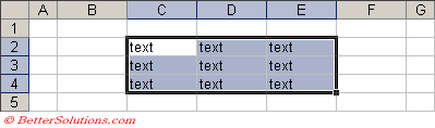
When you have a "clean" worksheet the following code returns the correct last cell "E4".

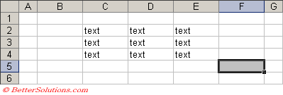
However this property does not just include cells that contain actual data but also any cells that have been formatted.
For example if we run the same code on the following worksheet the last cell is "F5".

Using SpecialCells(xlCellTypeLastCell)

This is the equivalent of using Ctrl+End and therefore also relies on the "UsedRange" property.
The same is true for the xlCellTypeLastCell argument which can be used with the SpecialCells property.

llastrow = Range("A1").SpecialCells(XlCellType.xlCellTypeLastCell).Row 
Debug.Print llastrow 

llastcolumn = Range("A1").SpecialCells(XlCellType.xlCellTypeLastCell).Column 
Debug.Print llastcolumn 

This also includes formatting in the range that is returned.
The xlLastCell constant is not documented because this constant was replaced in Excel 97 with the new xlCellType.xlCellTypeLastCell.
The following line of code does work but has only been included for backwards compatibility reasons.

llastrow = Range("A1").SpecialCells(xlLastCell).Row 

The macro recorder will generate code with the xlLastCell constant which adds to the confusion.

Using Cells.Find

Another popular approach which can be used to obtain the last "populated" row and column is to use the Cells.Find method.
This method searches backwards first by row and then by column from the top left cell.
The last row is the last visible row taking Filtering into account, but is not impacted by Manually Hidden Rows or collapsed Grouping.
The last column is the last visible column taking Manually Hidden Columns into account, but is not impacted by collapsed Grouping.

llastrow = ActiveSheet.Cells.Find(What:="*", _ 
                                  After:=ActiveSheet.Range("A1"), _ 
                                  SearchOrder:=XlSearchOrder.xlByRows, _ 
                                  SearchDirection:=XlSearchDirection.xlPrevious).Row 
Debug.Print llastrow 

Dim oRange As Range 
Set oRange = Range("A1:E200") 
llastrow = oRange.Find(What:="*", SearchOrder:=xlByRows, SearchDirection:=xlPrevious).Row 
Debug.Print llastrow 

llastcolumn = ActiveSheet.Cells.Find(What:="*", _ 
                                     After:=ActiveSheet.Range("A1"), _ 
                                     SearchOrder:=XlSearchOrder.xlByColumns, _ 
                                     SearchDirection:=XlSearchDirection.xlPrevious).Column 
Debug.Print llastcolumn 

llastcolumn = oRange.Find(What:="*", SearchOrder:=xlByColumns, SearchDirection:=xlPrevious).Column 
Debug.Print llastcolumn 

Using End(xlUp)

Use the following to obtain the address of the last non-empty cell in column "A".
The last row is the last visible row taking into account Filtering, Manually Hidden Rows and collapsed Grouping.

llastrow = Range(Range("A65536").End(xlDirection.xlUp).Address).Row 
llastrow = Range("A" & Rows.Count).End(xlUp).Row 
Debug.Print llastrow 

Last Column in a Range

Use the following to obtain the last column in a range.

Dim oRange As Range 
Set oRange = Range("A1:E200") 
llastcolumn = oRange(oRange.Rows.Count, oRange.Columns.Count).Column 
Debug.Print llastcolumn 

Application.GoTo

Selects any range or Visual Basic procedure in any workbook, and activates that workbook if it's not already active.
expression.Goto(Reference, Scroll)
Reference Optional Variant. The destination. Can be a Range object, a string that contains a cell reference in R1C1-style notation, or a string that contains a Visual Basic procedure name. If this argument is omitted, the destination is the last range you used the Goto method to select.
Scroll Optional Variant. True to scroll through the window so that the upper-left corner of the range appears in the upper-left corner of the window. False to not scroll through the window. The default is False.
This method differs from the Select method in the following ways:
     ● If you specify a range on a sheet that's not on top, Microsoft Excel will switch to that sheet before selecting. (If you use Select with a range on a sheet that's not on top, the range will be selected but the sheet won't be activated).
     ● This method has a Scroll argument that lets you scroll through the destination window.
     ● When you use the Goto method, the previous selection (before the Goto method runs) is added to the array of previous selections (for more information, see the PreviousSelections property). You can use this feature to quickly jump between as many as four selections.
     ● The Select method has a Replace argument; the Goto method doesn't.
This example selects cell A154 on Sheet1 and then scrolls through the worksheet to display the range.

Application.Goto Reference:=Worksheets("Sheet1").Range("A154"),     scroll:=True 

Range.Find Method

Finds specific information in a range, and returns a Range object that represents the first cell where that information is found.
Returns Nothing if no match is found. Doesn't affect the selection or the active cell.
The settings for LookIn, LookAt, SearchOrder, and MatchByte are saved each time you use this method.
If you don't specify values for these arguments the next time you call the method, the saved values are used.
Setting these arguments changes the settings in the Find dialog box, and changing the settings in the Find dialog box changes the saved values that are used if you omit the arguments.
To avoid problems, set these arguments explicitly each time you use this method.
You can use the FindNext and FindPrevious methods to repeat the search.

When the search reaches the end of the specified search range, it wraps around to the beginning of the range. To stop a search when this wraparound occurs, save the address of the first found cell, and then test each successive found-cell address against this saved address.
To find cells that match more complicated patterns, use a For Each...Next statement with the Like operator. For example, the following code searches for all cells in the range A1:C5 that use a font whose name starts with the letters "Cour". When Microsoft Excel finds a match, it changes the font to Times New Roman.

Finding any matching values

When searching a large range of cells it is significantly faster to search a column and spin down the rows as opposed to a row and spin through all the columns.

Dim rgeRange As Range 

rgeRange = Cells.Find(What:=MyValue) 
If Not rgeRange Is Nothing Then 
   Cells.Find(What:=MyValue _ 
              After:=Range("C2"), _ 
              LookIn:=xlFindLookIn.xlValues, _ 
              LookAt:=xlLookAt.xlPart, _ 
              SearchOrder:=xlSearchOrder.xlByRows, _ 
              SearchDirection:=xlSearchDirection.xlNext, _ 
              MatchCase:=False).Activate 
End If 

What - The data you want to search for (String)
After - A single cell representing the cell to start searching from
LookIn - The type of data to search.
LookAt - Whether the search is against the whole string or part of the string.
SearchOrder - The order in which to search the range.
SearchDirection - The search direction when searching a range.
MatchCase - True or False to match the case
MatchByte - True to match double byte characters match only
SearchFormat - True to use the Application.FindFormat options.

Finding and selecting the Maximum Value in a Range

Sub GoToMax 
Dim WorkRange As Range 

If TypeName(Selection) <> "Range" Then Exit Sub 

If Selection.Cells.Count = 1 Then 
'set it to the whole worksheet
   Set WorkRange = ActiveSheet.Cells 
Else 
   Set WorkRange = Selection 
End If 

MaxVal = Application.WorksheetFunction.Max(WorkRange) 

'find it and select it
On Error Resume Next 
WorkRange.Find(What:=MaxVal, _ 
               After:=WorkRange.Range("A1"), _ 
               LookIn:=xlValues, _ 
               LookAt:=xlLookAt.xlPart, _ 
               SearchOrder:=xlSearchOrder.xlByRows, _ 
               SearchDirection:=xlSearchDirection.xlNext, _ 
               MatchCase:=False).Select 

If Err <> 0 Then MsgBox("Max value was not found: " & MaxVal) 
?? 

End Sub 

Finding any merged cells

Public Sub BET_Find_MergedCells() 
Dim rngCell As Range 
Dim stemp As String 

   stemp = "" 
   For Each rngCell In Selection 
      If rngCell.MergeCells = True Then 
         stemp = stemp & rngCell.Address & " " 
      End If 
   Next rngCell 
   Call MsgBox(Left(stemp, Len(stemp) - 1)) 
End Sub 

Finding Unique Items

This function will return the unique items in an array. Used to find the unique items in a column of Excel data.

Function UniqueItems(ArrayIn, Optional Count As Variant) As Variant 
'   Accepts an array or range as input
'   If Count = True or is missing, the function returns the number of unique elements
'   If Count = False, the function returns a variant array of unique elements
    Dim Unique() As Variant ' array that holds the unique items  
    Dim Element As Variant 
    Dim i As Integer 
    Dim FoundMatch As Boolean 
'   If 2nd argument is missing, assign default value
    If IsMissing(Count) Then Count = True 
'   Counter for number of unique elements
    NumUnique = 0       
'   Loop thru the input array
    For Each Element In ArrayIn 
        FoundMatch = False 
'       Has item been added yet?
        For i = 1 To NumUnique 
            If Element = Unique(i) Then 
                FoundMatch = True 
                GoTo AddItem '(Exit For-Next loop)  
            End If 
        Next i 
AddItem: 
'       If not in list, add the item to unique list
        If Not FoundMatch Then 
            NumUnique = NumUnique + 1 
            ReDim Preserve Unique(NumUnique) 
            Unique(NumUnique) = Element 
        End If 
    Next Element 
'   Assign a value to the function
    If Count Then UniqueItems = NumUnique Else UniqueItems = Unique 
End Function 

Offset Method

Range.Offset(RowOffset, ColumnOffset)
This method returns range that is offset to a range object.
This method does not change the active range (unlike the Select and Activate methods).
This enters the number 15 in the cell directly below and to the right of the active cell.

ActiveCell.Range("B2").Value = 15 

The preferred method though is to use the Offset property.

ActiveCell.Offset(rowindex, columnindex).Value = 15 
ActiveCell.Offset(1, 1).Value = 15 
ActiveCell.Offset(1, -2).Select 
Range(ActiveCell.Offset(1). ActiveCell.Offset(1).End(xlDirection.xlDown)).Select 
ActiveCell.Offset(0, 1).Value = "some text" 

Using the Offset position (0, 0) will refer to the active cell.

ActiveCell.Offset(0, 0).Value = "some text" 
Range("B2").Offset(4, 4).Value = 20 

If you try to Offset to a cell which has in invalid column or row number then an error will be generated.

Referring to the Row Above

Range("B2").Offset(1,0).Address = "B1" 
Range("B2").Offset(1).Address = "B1" 

Referring to the Row Below

Range("B2").Offset(1,0).Address = "B3" 
Range("B2").Offset(1).Address = "B3" 

Referring to the Next Column

Range("B2").Offset(0, 1).Address = "C2" 
Range("B2").Offset(, 1).Address = "C2" 

Referring to the Previous Column

Range("B2").Offset(0, 1).Address = "A2" 
Range("B2").Offset(, 1).Address = "A2" 

Resize Method

This allows you to alter the size of a range

Range("A1").Resize(2,3) = C2 

expression.Resize(RowSize, ColumnSize)

RowSize - The number of rows in the new range. If this argument is omitted, the number of rows in the range remains the same.
ColumnSize - The number of columns in the new range. If this argument is omitted, the number of columns in the range remains the same.
Both of these arguments are optional and if omitted then the range stays the same.
This example resizes the selection on Sheet1 to extend it by one row and one column.

Worksheets("Sheet1").Activate 
numRows = Selection.Rows.Count 
numColumns = Selection.Columns.Count 
Selection.Resize(numRows + 1, numColumns + 1).Select 

This example assumes that you have a table on Sheet1 that has a header row. The example selects the table, without selecting the header row. The active cell must be somewhere in the table before you run the example.

Set tbl = ActiveCell.CurrentRegion 
tbl.Offset(1, 0).Resize(tbl.Rows.Count - 1, _ 
    tbl.Columns.Count).Select 

or

Dim inoofcolumns As Integer 
Dim lnoofrows as Long 

inoofcolumns = ActiveCell.CurrentRegion.Columns.Count 
ActiveCell.CurrentRegion.Offset(1,0).Resize(lnoofrows - 1, inoofcolumns).Select 

Evaluate Method

You can also use the following abbreviations although they are not encouraged.
This method can be used to generate references to Range objects and also for calculating worksheet formulas.
The normal syntax is as follows:

Application.Evaluate("Expression") 

There are also several shortcut formats to this method as well.

Evaluate("Expression") 

You can also remove the quotes and surround the expression with square brackets.

[Expression] 

Calculating Formulas

The Expression can be any valid worksheet calculation, with or without the equal sign on the left.
The worksheet calculations can include worksheet functions that are not made available to VBA using the WorksheetFunction object.
The worksheet calculations can also be array formulas.
For example the ISBLANK worksheet function is not accessible using WorksheetFunction object because VBA has the equivalent IsEmpty() function.
The following two lines of code are equivalent.

Call MsgBox(Evaluate("=ISBLANK(A1)") 
MsgBox [ISBLANK(A1)] 

The advantage of using the first technique is that the worksheet formula string can be generated using code making it more flexible.

Manipulating a Range

The following two lines of code select the range of cells "A1:D4".

Range("A1:D4").Select 
[A1:D4].Select 

Application.Evaluate("A4").Value = "some text" 
Evaluate("A4").Value = "some text" 
A4.Value = "some text" 
[A4].Value = "some text" 

This expression could it fact be simplified even more since the default property for a Range object is Value.
Using the default properties is definitely not recommended.

[A4] = "some text" 

You can also use this technique to quickly refer to cells using Named Ranges.

[Named_Range].Select 
[Named_Range] = "some text" 

Quick Arrays

The Evaluate method can also be used to quickly obtain an array of numbers.

Dim arValues As Variant 
arValues = Application.Evaluate("Row(1:50)")  =  {1,2,3, .. 50} 

Similarly you can use this technique to quickly insert a sequence of numbers into a range of cells.

Range("B1:B50").Value = Application.Evaluate("Row(1:50)") 

Other Named Objects

Evaluate can also be used with other named objects, such as drawing elements.
It can also be used with Named Ranges.

AutoFill - Filling a Range Down

You do not have to select the cells first

objRange.Auto Fill(Destination:=Range("B2"), _ 
                  Type:=xlAutoFillType.xlFillDefault) 

The Destination is the range of cells to be filled. This cell range must include the actual source data in order to create the Auto Fill.
If the Type argument is left blank or you choose xlFillDefault then Excel will attempt to select the most appropriate fill type based on the source data.

Example when cell contains values

Example when cell contains formulas

One potential problem with the Auto Fill method is that when it is executed, the formula in the source cell is copied, with changes to other cells.
However the value of the source cell is also copied, but without changes.
So if autocalculation is switched off, the formulas will be correct but the values will be incorrect.
This can be overcome by invoking a Calculate method after the Auto Fill has been executed.

Application.Calculate 

Filling Down with Values

Fills down from the top cell or cells in the specified range to the bottom of the range.
The contents and formatting of the cell in the top row of a range are copied into the rest of the rows in the range.

Selection.FillDown 

This example copies the contents in cell "A1" down to the whole range "A2:A10".

Range("A1:A10").FillDown 

Filling Down with Formulas

Range("C1").Formula = "=A1+B1" 
Range("C1:C7").FillDown 

Restricting the Scroll Area of a worksheet

It is possible to restrict the scroll area of a worksheet by using the ScrollArea property of a worksheet object.
Open the workbook and select the worksheet you want to restrict the scroll area for.
Defining a specific scrollarea though will prevent the user from being able to select the row and column headings.
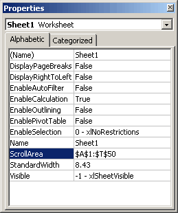
Display the Control Toolbox toolbar and select the Properties button.
This will display the Properties window for that specific worksheet allowing you to define a scroll area.

Alternatively you could use the following line of VBA code:

Sheets(1).ScrollArea = "A1:H20" 

To reset the scroll area afterwards, set the scroll area back to being the whole worksheet.

Sheets(1).ScrollArea = Sheets(1).Cells.Address 

Any cells outside this area cannot be selected.

Worksheets(1).ScrollArea = "A1:E20" 

Set this property to an empty string to enable cell selection on the entire worksheet.

Hyperlinks

Range("B2").Hyperlinks.Add(Anchor:= 
                    Address:= 
                   TextToDisplay:= 

Anchor - This can either be a Range or a Shape.
Address - The address of the hyperlink.
SubAddress - The subaddress of the hyperlink
This can be used to create links to cells in the same workbook (eg cells and named ranges)

ScreenTip - The text to display when you hover over with the mouse.
TextToDisplay - The text to display as the hyperlink.

ActiveWorksheet.Hyperlinks.Delete 

ActiveWorkbook.FollowHyperlink 
   Address:="https://bettersolutions.com" 
   NewWindow:=True 

Removing all Hyperlinks

Public Sub RemoveAllHyperlinks() 
Dim objworksheet As Worksheet 
Dim objhyperlink As Hyperlink 
Dim lhypercount As Long 
Dim answer 

'Set objworksheet = Selection.Parent
answer = MsgBox("Do you want to remove " & Selection.Cells.Hyperlinks.Count & " hyperlinks ?", _ 
                vbQuestion + vbYesNo) 
                
If answer = vbNo Then 
   Exit Sub 
End If 

For lhypercount = Selection.Cells.Hyperlinks.Count To 1 Step -1 
   Set objhyperlink = Selection.Cells.Hyperlinks(lhypercount) 
   objhyperlink.Delete 
Next lhypercount 
   
   Call MsgBox("done") 
End Sub 

Private Sub Worksheet_FollowHyperlink(ByValTarget As Hyperlink) 
   Call Hyperlink_Activate(Target) 
End Sub 

Public Sub Hyperlink_Activate(ByVal objHyperlink As Hyperlink) 
Dim sScreenTip As String 
   sScreenTip = objHyperlink.ScreenTip 

   Select Case sScreenTip 
      Case "MacroName" 
           'do something
        'maybe even update the ScreenTip
      objHyperlink.ScreenTip = "Blah blah" 

   End Select 

End Sub 

This can be used to invoke an action or a macro
To create a hyperlink that just takes you to another part of the workbook
right click the cell, choose hyperlink
Select "place in the document" button on the left
In the "type the cell reference" add the cell you want to contain the link
This ensures that the selection doesn't change when the user presses the link.
This links the cell to itself

The following events are raised:
Application.SheetFollowHyperlink
Workbook.SheetFollowHyperlink
Worksheet.FollowHyperlink