Comparing Lists

This example shows you how to identify particular items in a list.
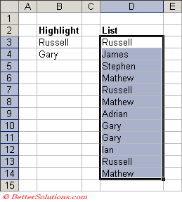
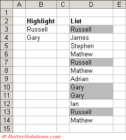
When a particular item or category is entered in column "B", the conditional format automatically highlights all the corresponding entries in the list in column "D".
Select the cells you want to apply the conditional formatting to, in this case "D3:D14".

Enter Conditions

Press (Format > Conditional Formatting) to display the Conditional Formatting dialog box.
Select the "Formula is" in the first drop-down list and enter the formula "=COUNTIF($B$B,D3)".

Press OK to apply the conditional formatting.

Getting the Total

You could also return the total number of items that match in the list by using an Array Formulas.

Highlight Differences

indicate the items in one list that appear in another
Start by selecting the OldList range.
In the Conditional Formatting dialog box, use the drop-down list to choose Formula is.
Enter this formula: =COUNTIF(NewList,B9)=0
Click the Format button and specify the formatting to apply when the condition is true (a yellow background in this example).

The cells in the NewList range will use a similar conditional formatting formula.

Select the NewList range.
In the Conditional Formatting dialog box, use the drop-down list to choose Formula is.
Enter this formula: =COUNTIF(OldList,E9)=0
Click the Format button and specify the formatting to apply when the condition is true (a green background in this example).