Weekends

This example shows you how to identify the weekends when you have a list of dates.
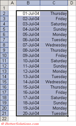
Select the cells you want to apply the conditional formatting to, in this case "B2:C21".

Enter Conditions

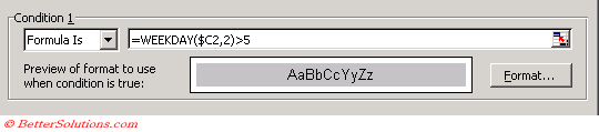
Press (Format > Conditional Formatting) to display the Conditional Formatting dialog box.
Select the "Formula is" in the first drop-down list and enter the formula "=WEEKDAY($C2,2)>5".
For more examples of this function please refer to the WEEKDAY page.
You can either type the cell references or you can use your mouse to select the cell ranges.
When you want to refer to the active cell you need to refer to the first cell in the highlighted range.

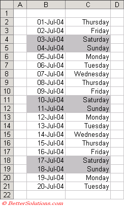
Press OK to apply the conditional formatting.

This formula will actually highlight any empty cells as well since the WEEKDAY() function returns the number 7 for a blank value.
To avoid shading any empty cells you could use the following formula "IF(ISBLANK(B2),"",WEEKDAY($C2,2)>5)".