Duplicate Values

This example shows you how to use Conditional Formatting to highlight all the duplicate entries in a list.
If you have a large list of data you may find it useful to be able to identify any duplicate entries in a list.
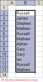
Select the cells you want to apply the conditional formatting to, in this case "B2:B13".

Enter Conditions

Highlight the range of cells
Select (Home, Conditional Formatting)(Highlight Cells Rules > Duplicate Values)
Any duplicate values will be highlighted allowing you to sort all the shaded cells to the top.
Click on a cell with shading
Right click and select (Sort > Put Selected Cell Colour on Top)
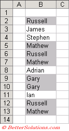
When duplicate is found both occurrences are highlighted.

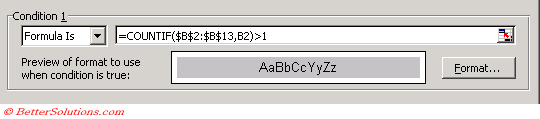
Press (Format > Conditional Formatting) to display the Conditional Formatting dialog box.
Select the "Formula is" in the first drop-down list and enter the formula "COUNTIF($B$2:$B$13,B2)>1".
You can either type the cell references or you can use your mouse to select the cell ranges.
You can also use the F4 key to toggle between the absolute and relative cell references.
When using functions and especially cell references it is important to understand the significance between using absolute and relative references.

Press OK to apply the conditional formatting.

If you wanted to highlight the values that appeared twice you could change the formula to "=COUNTIF($B$2:B$13,B2)=2".
If you wanted to highlight the values that appeared more than twice you could change the formula to "=COUNTIF($B$2:B$13,B2)>2".

Other Alternatives

using the unique records only on Advanced Filter - inc link
use COUNTIF function to count the number of instances, COUNTIF(A$1:A1,A2) = 0
Use a pivot table