Error Values

This example shows you how to apply conditional formatting that will highlight any cells that contain errors.
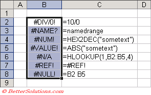
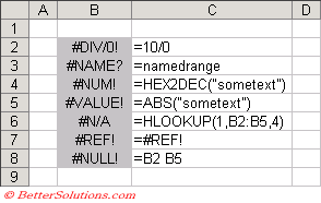
Select the cells you want to apply the conditional formatting to, in this case "B2:B8".

Enter Conditions

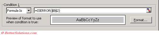
Press (Format > Conditional Formatting) to display the Conditional Formatting dialog box.
Select the "Formula is" in the first drop-down list and enter the formula "=ISERROR($B$2)".
You can either type the cell reference or you can use your mouse to select the cell "B2".
If you only wanted to highlight the "#N/A" on the worksheet you could use the formula "=ISNA(B2)
Click the Format button to apply your specific formatting, in this case we are just applying a grey background.

Press OK to apply the conditional formatting.

Removing Errors

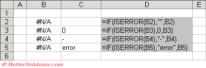
It is sometimes necessary to not display any error values on a worksheet and this can be achieved by using the IF() function.
You can use the IF() function to detect is there is an error and to return either a blank, a zero or something else.

It is also possible to hide any errors from your printouts by changing the (File > Page Setup)(Sheet tab, "Cell errors as") option.