INDEX Function

The INDEX function returns the value from a cell range which is the intersection of a row and a column.
The tooltip for this function can be seen below and looks quite complicated.
In fact before we try and understand this function we need to make a small modification to the tooltip.

The reference syntax for this function is the one used in 99% of cases, so lets assume it's the only one that exists.
Having the other one displayed in the tooltip is unnecessary and causes users a lot of confusion.

Return a Single Value (in a table)

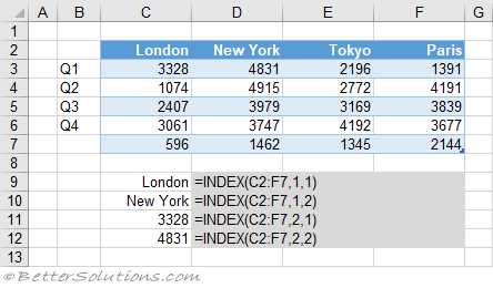
You can return a single value from a range by passing in a row number and a column number.
The row and column numbers are the "relative" numbers to the range and not the literal row and column numbers.
For most of us this is the only reason that we need to use this function.

Return a Single Value (in a column)

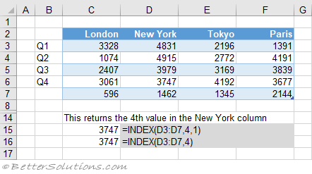
You can return the value that is at a certain position in a single column reference.
When the reference is just a single column, the 'column num' is ignored and is optional.

Return a Single Value (in a row)

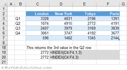
You can return the value that is at a certain position in a single row reference.
When the reference is just a single row, it is possible to exclude the 'row_num' and just submit the 'column_num'.
The formula in row 20 only has two arguments, the cell reference and the column number.
This would be considered very bad practice though and would introduce a lot of unnecessary confusion.

Return the Same Value (from multiple tables)

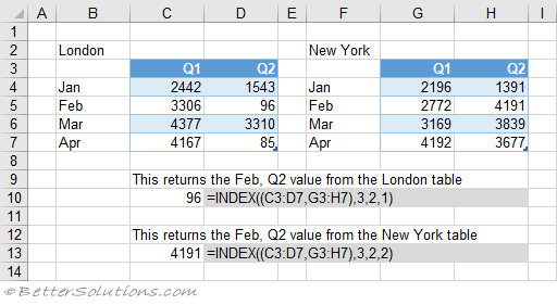
You can return the same value from a number of different tables.
These tables can be in non adjacent cells (and even on different worksheets).
It is possible to return the same relative cell from different tables by making use of the optional 'area_num' argument.

Return Multiple Values

For the more advanced users, you can use this function to return multiple values from a range.
This might be useful if you have a large table and want to display a number of consecutive cells.
In these examples the function is returning 4 values.
When you set the 'column_num' to zero, the entire row is returned.
You must select all the cells first and the formula must be entered as an Array Formula using (Ctrl + Shift + Enter).

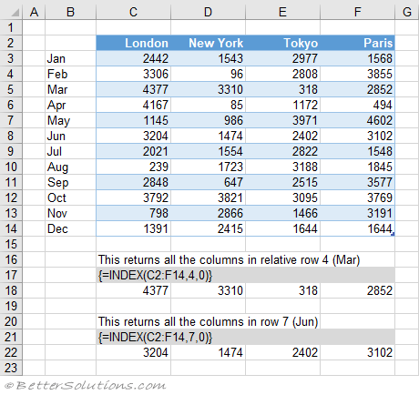When you set the 'row_num' to zero the entire column is returned.

When "column_num" and "row_num" are zero, the entire table is returned.

Non Adjacent Cells

If "reference" contains non adjacent cells, the cell ranges must be enclosed in parentheses.
If "area_num" is too small or too large, then #REF! is returned.
=INDEX((A1:B7,D1:D7,G1:H7),3,2,1) = 30
=INDEX((A1:B7,D1:D7,G1:H7),3,2,3) = 3000

Using an Array Constant

This function can also accommodate the use of array constants.
=INDEX(array, row_num, [column_num])
=INDEX({1,2,3,4,5,6,7},2) = 2
=INDEX({1,2;3,4;5,6;7,8},2,2) = 4

Cell References Instead

This function can also return a cell reference instead of the cell value.
=CELL("width",INDEX(A1:B2,1,2)) - index returns the cell reference
=2*INDEX(A1:B1,1,2) - returns the actual value

Important

When we talk about the MATCH / INDEX equivalent of a VLOOKUP, the INDEX function is returning a single value.