Two Way Lookup

A two-way lookup is when you need to find a particular row in one column and return a different value from the same row.
This type of lookup can be used on tables that just have header columns.
This type of lookup can be used on tables that have row headers in the first column.

There are lots of different functions and formulas we can use to do this and choosing the right one will depend on the following:
(1) Is your lookup column always the first column in the table.
(2) Is this a "one off" task or something you will need to do regularly.
(3) Will you want to quickly return data from a different column.
(4) Will the table always have exactly the same columns in exactly the same order.
(5) Do you want to use more than one criteria (ie multiple columns) to identify a specific row.
Notice that some of these functions use column numbers, some use ranges and some use column headers.

One criteria using a Fixed Column - XLOOKUP

We can use the XLOOKUP function to perform a two-way lookup.
The formula in cell "F3" returns the Sales corresponding to the criteria "Country=Japan".
The formula in cell "F7" returns the City corresponding to the criteria "Country=Japan".
The formula in cell "F11" returns the City corresponding to the criteria "Country=United States".

=XLOOKUP(G2,B3:B14,C3:C14)

One criteria using a Fixed Column - INDEX, MATCH

We could use the INDEX and MATCH functions.
The formula in cell "F3" returns the Sales corresponding to the criteria "Country=Japan".
The formula in cell "F7" returns the City corresponding to the criteria "Country=Japan".
The formula in cell "F11" returns the City corresponding to the criteria "Country=France".

=INDEX(C3:C14,MATCH(G2,B3:B14,0))

One criteria using a Fixed Column - VLOOKUP

You could use the VLOOKUP function.
This function will only work when the value you are looking up is in the first column.
The formula in cell "F3" returns the Sales corresponding to the criteria "Country=Japan".
The formula in cell "F7" returns the City corresponding to the criteria "Country=Japan".
The formula in cell "F11" returns the City corresponding to the criteria "Country=Germany".

=VLOOKUP(G2,B2:D14,2,FALSE)

One criteria using a Fixed Column - VLOOKUP, CHOOSE

You can combine the VLOOKUP function and the CHOOSE function when the value you are looking up is not in the first column.
Try and avoid using this combination because the formula looks complicated and is not very easy to understand.
The CHOOSE function provides a way of returning the cell ranges as arrays.

=VLOOKUP("myvalue",CHOOSE({1,2},B1:B10,C1:C10),2,0)

One criteria using a Fixed Column - OFFSET, MATCH

You could use the OFFSET and MATCH functions.
Try and avoid using this combination because OFFSET is volatile function.
Volatile functions recalculate every time any cell in the workbook changes.

One criteria using a Fixed Column - LOOKUP

You could use the LOOKUP function.
Try and avoid using this functon because the lookup column has to be sorted into ascending order.
This table has been sorted by Country.

One criteria using a Fixed Column - SUMPRODUCT

You could use the SUMPRODUCT function.
Try and avoid using this function because this function can only be used to return numbers (not text).
You must include the double unary/negative prefix.

Using Column Headers Instead

Instead of using a fixed column (either by number or by range) it is possible to use a column header instead (in this case City).
This can be useful when you get sent the same table regularly but the order of the columns may change.

One criteria using a Column Header - XLOOKUP, XLOOKUP

=XLOOKUP(G2,B3:B14,XLOOKUP(G3,B2:D2,B3:D14))

One criteria using a Column Header - INDEX, MATCH, MATCH

=INDEX(B3:D14,MATCH(G2,B3:B14,0),MATCH(G3,B2:D2,0))

One criteria using a Column Header - VLOOKUP, HLOOKUP

link - mbaexcel.com/excel/how-to-use-the-vlookup-hlookup-combination-formula/

=VLOOKUP(C5, C15:G20, HLOOKUP(D5, C13:G14, 2, FALSE), FALSE)

One criteria using a Column Header - VLOOKUP, MATCH

=VLOOKUP(G2,B3:D14,MATCH(G3,B2:D2,0),FALSE)

One criteria using a Column Header - HLOOKUP, MATCH

=HLOOKUP(G3,B2:D14,MATCH(G2,B2:B14,0),FALSE)

One criteria using a Column Header - OFFSET, MATCH, MATCH

Not recommended

One criteria with Named Ranges and INDIRECT

Not recommended
This uses Create from Selection
formula = INDIRECT("February") INDIRECT("Chicago")
and then uses Range Intersection

Two Criteria

Also known as 2 Dimensional lookups

Two criteria with an Additional Column

A quick solution is to add an additional column which is a concatenation of the columns you want to match
The formulas below can be used when you do not want to insert an additional column.
For very large data sets you should always insert an additional (helper) column to avoid performance problems.

Two criteria using Fixed Columns - INDEX, MATCH, IF

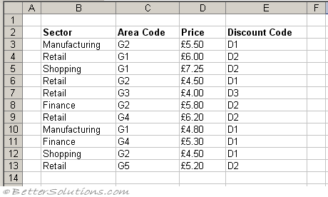
Lets assume we have got the following table and we want to return the Price corresponding to the sector "Retail" and the area code "G3".

=INDEX(D3:D13,MATCH("Retail",IF(C3:C13="G3",B3:B13),0))

Two criteria using Fixed Columns - INDEX, MATCH and Multiplication

=INDEX(D3:D13,MATCH(1,("B3:B13="Retail")*(C3:C13="G3"),0))

Two criteria using Fixed Columns - INDEX, MATCH and String Concatenation

This is often a preferred method as it does not include nested IF functions.

=INDEX(D3:D13,MATCH("Retails"&"G3",B3:B13&C3:C13,0))