Comparing Columns

The XMATCH function can be used to check if a value in one column exists in another column.
The data does not have to be sorted.

Using XMATCH

You can use the XMATCH to return whether an item exists in a list or not.
The XMATCH function can be combined with the ISNUMBER function to return True or False.
If there is an exact match this formula will return True.
If the item does not exist in the full list this formula will return False.

=ISNUMBER(XMATCH(C3,$B$3:$B$14,0)) 

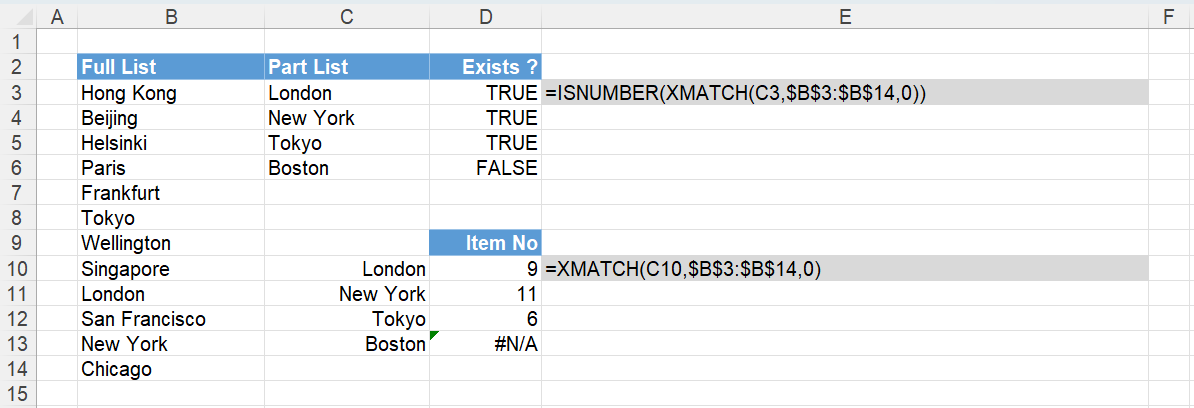The XMATCH function will return the position in the list if the item can be found.
The XMATCH function will return #N/A if the item cannot be found.
The ISNUMBER function can be used to change the position number into a True and the #N/A into a False.

Using XMATCH (case sensitive)

The XMATCH function is not case sensitive.
To perform a case sensitive lookup you can combine the XMATCH function with the EXACT function.
If there is an exact match this formula will return True.
If the item does not exist in the full list this formula will return False.

=ISNUMBER(XMATCH(TRUE,EXACT($B$3:$B$14,C3),0)) 

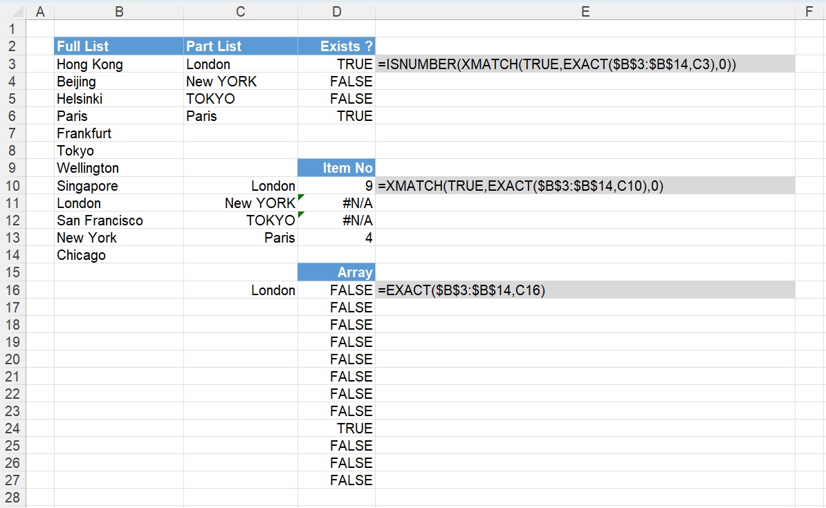The EXACT function will return an array of True or False values based on a case sensitive comparison.
If there is an exact match this array will contain the value True.
The XMATCH function will return the position in the list if the item can be found.
The XMATCH function will return #N/A if the item cannot be found.
The ISNUMBER function can be used to change the position number into a True and the #N/A into a False.

Using MATCH

Instead of using the XMATCH function we could use the MATCH function.
Instead of using the ISNUMBER function we could use the ISERROR function and the NOT function.
If there is an exact match this formula will return True.
If the item does not exist in the full list this formula will return False.

=NOT(ISERROR(MATCH(C3, $B$3:$B$14, 0))) 

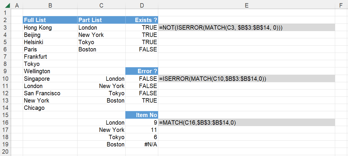The MATCH function will return the position in the list if the item can be found.
The MATCH function will return #N/A if the item cannot be found.
The ISERROR function can be used to change the position number into a False and the #N/A into a True.
The NOT function can be used to reverse the True and False.

Using MATCH (case sensitive)

The MATCH function is not case sensitive.
To perform a case sensitive lookup you can combine the MATCH function with the EXACT function.
Instead of using the ISERROR function we could use the ISNA function.
Instead of using the NOT function we could use the IF function.

=IF(ISNA(MATCH(TRUE,EXACT(C3:B14,A1),0)),FALSE,TRUE) 

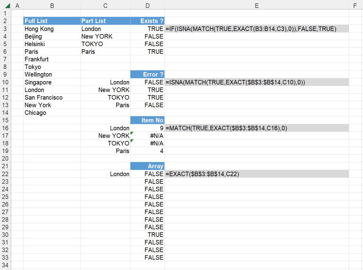The EXACT function will return an array of True or False values based on a case sensitive comparison.
If there is an exact match this array will contain the value True.
The MATCH function can then lookup the value True in this array and return its corresponding position in the list.
The MATCH function will return #N/A if the value True cannot be found in the array.
The ISNA function can be used to change the position number into a False and the #N/A into a True.
The IF function can be used to reverse the True and False.

Using VLOOKUP

You could use the VLOOKUP function with just a single column.
Try and avoid doing this because VLOOKUP was really designed to perform a two-way lookup across a table.
Here are a few more reasons to not use it.
(1) The MATCH function is faster than the VLOOKUP function.
(2) The MATCH formula is simpler than the VLOOKUP formula.

=NOT(ISNA(VLOOKUP(C3,B3:B14,1,False))) 

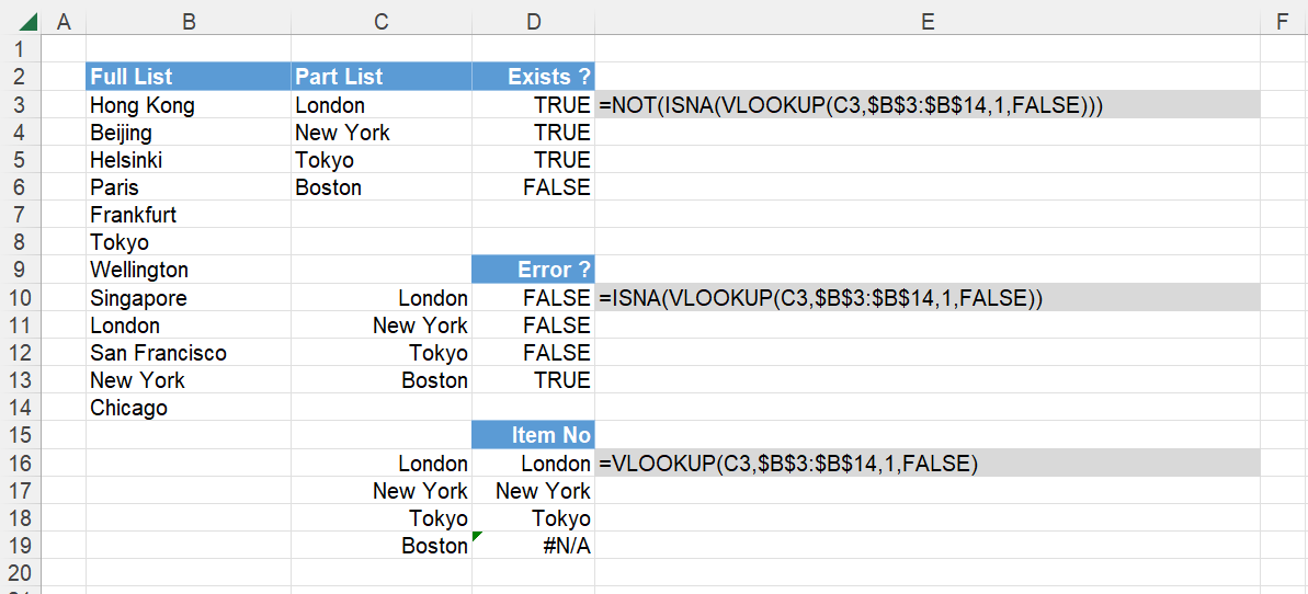The VLOOKUP function will return the matched value if the item can be found.
The VLOOKUP function will return #N/A if the item cannot be found.
The ISNA function can be used to change the matched item into a False and the #N/A into a True.
The NOT function can be used to reverse the True and False.