HLOOKUP Function

The HLOOKUP function returns the value in a row that matches a value in the top row of a table
XLOOKUP was added in Excel 2021 to replace this function.
This looks up a value in the first row of a table and returns the value in the same column but in a different row.
This function is not case sensitive.

Return the Exact Match (unique values)

When the "range_lookup" argument is FALSE an exact match is found.
If there is more than one occurrence, the first occurrence is found.
The table does not have to be sorted when looking for an exact match.

Return the Exact Match (item does not exist)

When the "lookup_value" is not in the list, #N/A is returned.
When the "range_lookup" argument is FALSE an exact match is found.
The table does not have to be sorted when looking for an exact match.

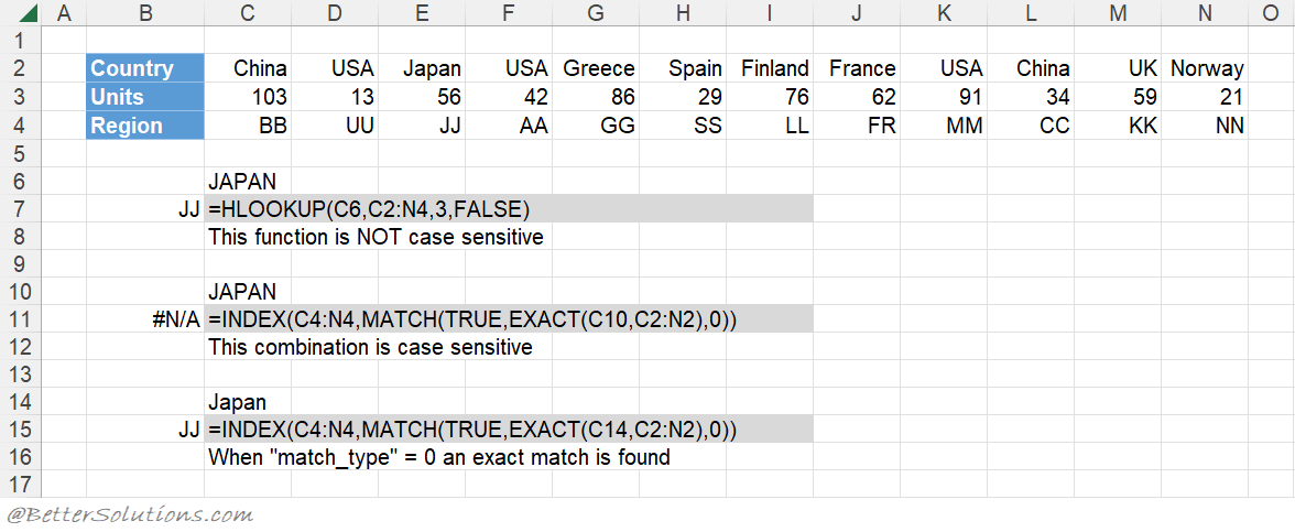
Return the Exact Match (case sensitive)

The HLOOKUP function is not case sensitive.
This means that upper case and lower case characters are equal (for example Japan = JAPAN).
You can perform a case sensitive lookup by using the INDEX, MATCH and EXACT functions.
The "0" passed to the MATCH function means that it will find an exact match.

Return the Exact Match (first occurrence, sorted or not sorted)

This function will always return the first occurrence, starting on the left.
When the "range_lookup" argument is FALSE an exact match is found.
The table does not have to be sorted to return the first occurrence.

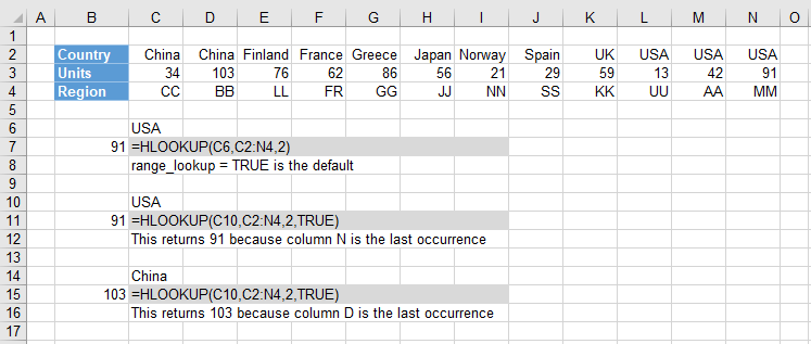
Return the Exact Match (last occurrence, sorted)

The last occurrence can be achieved when the lookup row is sorted into ascending order.
The table has been sorted by Country into ascending order.

Return the Exact Match (last occurrence, not sorted)

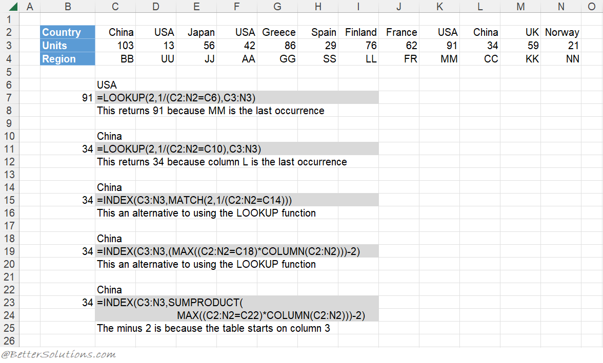
You can get the last occurrence when the "lookup_value" row is not sorted by using the LOOKUP function.
The LOOKUP function uses an array of cell values and its closest match logic to find the last match.
The array eventually contains either 1's or error values and because the "lookup_value" is 2 it will return the position of the last 1 in the array.
You could use the INDEX and MATCH functions as an alternative.
You could use the INDEX, MAX and COLUMN as another alternative.
You could use the SUMPRODUCT function as another alternative.

Return the Exact Match (with wildcard *)

An asterisk (*) matches any sequence of characters.
The "range_lookup" argument must be FALSE.
You can have an asterisk as the first character.

Return the Exact Match (with wildcard ?)

A question mark (?) matches any single character.
The "range_lookup" argument must be FALSE.
You can have a question mark as the first character.

Return the Exact Match (multiple criteria)

When you want to return a value in the same column after finding matching values in 2 (or more) rows.

Return the Next Smallest

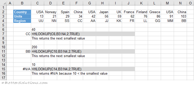
The next smallest value can achieved when the lookup column is sorted into ascending order.
When the "range_lookup" argument is TRUE the nearest smallest value is found.
When the "range_lookup" argument is TRUE the table must be sorted.
The table has been sorted by Units into ascending order.

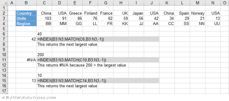
Return the Next Largest

The next largest value can be achieved using the INDEX and MATCH combination.
The table has been sorted by Units into descending order.
The "-1" passed to the MATCH function means that it will find the smallest value that is greater than the lookup value.

Combining with MATCH

A two way lookup can be achieved using a HLOOKUP and MATCH combination.
A two way lookup is when you return the intersection of a matching column with a matching row.

Important

When no match is found and you want to return approximate values, the first row of your table must be sorted in ascending order.
If you are searching for numbers then they must be formatted as numbers and not as text. If they are formatted as text they will be ignored.
This function can only be used to return values in rows below the lookup column.
The lookup row has to be the first row in the table.